Bias-Variance Tradeoff Matthieu R. Bloch h in a given set H that - PDF document

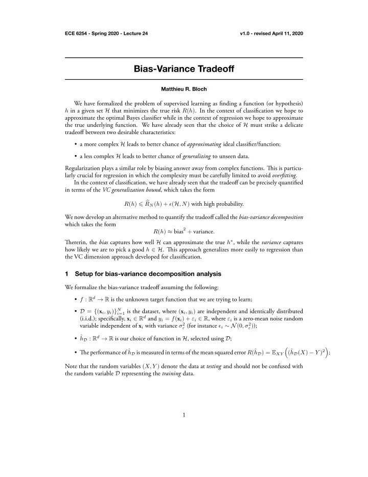
1 Regularization plays a similar role by biasing answer away from complex functions. Tiis is particu- ; We formalize the bias-variance tradeoff assuming the following: which takes the form We now develop an alternative method to quantify the tradeoff called the bias-variance decomposition in terms of the VC generalization bound , which takes the form In the context of classification, we have already seen that the tradeoff can be precisely quantified larly crucial for regression in which the complexity must be carefully limited to avoid overfitting . the VC dimension approach developed for classification. tradeoff between two desirable characteristics: approximate the optimal Bayes classifier while in the context of regression we hope to approximate We have formalized the problem of supervised learning as finding a function (or hypothesis) ECE 6254 - Spring 2020 - Lecture 24 v1.0 - revised April 11, 2020 Bias-Variance Tradeoff Matthieu R. Bloch h in a given set H that minimizes the true risk R ( h ) . In the context of classification we hope to the true underlying function. We have already seen that the choice of H must strike a delicate • a more complex H leads to better chance of approximating ideal classifier/function; • a less complex H leads to better chance of generalizing to unseen data. R ( h ) ⩽ � R N ( h ) + ϵ ( H , N ) with high probability. R ( h ) ≈ bias 2 + variance . Tiererin, the bias captures how well H can approximate the true h ∗ , while the variance captures how likely we are to pick a good h ∈ H . Tiis approach generalizes more easily to regression than 1 Setup for bias-variance decomposition analysis • f : R d → R is the unknown target function that we are trying to learn; • D = { ( x i , y i ) } N i =1 is the dataset, where ( x i , y i ) are independent and identically distributed (i.i.d.); specifically, x i ∈ R d and y i = f ( x i ) + ε i ∈ R , where ε i is a zero-mean noise random variable independent of x i with variance σ 2 ε (for instance ϵ i ∼ N (0 , σ 2 ε ) ); h D : R d → R is our choice of function in H , selected using D ; • ˆ � h D ( X ) − Y ) 2 � • Tie performance of ˆ h D is measured in terms of the mean squared error R (ˆ (ˆ h D ) = E XY Note that the random variables ( X, Y ) denote the data at testing and should not be confused with the random variable D representing the training data.

2 Tie last three terms turn out to be zero since . Tien, (1) (2) (3) (4) Var (5) (6) (7) Var with (8) and (9) (10) that we obtain. Tie model space represent, for instance, all the linear models while the regularized model represents the regularized models. Tie blue area represents the variance of the model while the orange area represents the variance of the regularized model. Tie regularized model offers a smaller variance at the expense of an increased bias. Lemma 1.1 (Bias-variance decomposition ) . Var ECE 6254 - Spring 2020 - Lecture 24 v1.0 - revised April 11, 2020 � � � � � � � � R (ˆ ˆ Bias (ˆ = σ 2 h D ( X )) 2 | X E D h D ) ε + E X h D ( X ) | X + E X �� �� 2 � � � � ˆ ˆ ˆ ≜ E D h D ( X ) − E D h D ( X ) h D ( X ) � � Bias (ˆ ˆ h D ( X )) ≜ E D h D ( X ) − f ( X ) � � Proof. For clarity, set ¯ ˆ h ( X ) ≜ E D h D ( X ) � � � � h D ( X ) − Y ) 2 �� R (ˆ (ˆ E D h D ) = E D E XY � � h D ( X ) − f ( X ) − ε ) 2 �� (ˆ = E D E Xε � � h ( X ) − f ( X ) − ε ) 2 �� (ˆ h D ( X ) − ¯ h ( X ) + ¯ = E D E Xε � h ( X )) 2 + (¯ h ( X ) − f ( X )) 2 + ε 2 (ˆ h D ( X ) − ¯ = E D E X E ε +2(ˆ h D ( X ) − ¯ h ( X ))(¯ h ( X ) − f ( X )) − 2(ˆ h D ( X ) − ¯ h ( X )) ε � − 2(¯ h ( X ) − f ( X )) ε Note that in (4) we have used the fact that D , X , and ε are independent. Notice that � h ( X )) 2 � � � �� (ˆ h D ( X ) − ¯ ˆ ≜ E X h D ( X ) | X E D E X E ε � h D ( X )) 2 � � h ( X ) − f ( X )) 2 � (¯ Bias (ˆ ≜ E X E D E X E ε � ε 2 � ≜ σ 2 E D E X E ε ε . � � � � � � (ˆ h D ( X ) − ¯ h ( X ))(¯ ˆ − ¯ h ( X ))(¯ h ( X ) − f ( X )) = E X ( E D h D ( X ) h ( X ) − f ( X )) E D E X = 0 � � � � �� (ˆ h D ( X ) − ¯ h D ( X ) − ¯ ˆ h ( X )) ε = E X h ( X ) E ε ( ε ) = 0 E D E X E ε E D � � � ¯ � (¯ h ( X ) − f ( X )) ε = E X h ( X ) − f ( X ) E ε ( ε ) = 0 . E D E X E ε ■ 2 Intuition behind the bias-variance tradeoff Tie intuition behind the bias-variance tradeoff is illustrated in Fig. 1. Tie gray area around the true function f represents the variance of the perception of the true resulting from the noisy samples

3 function Model space Regularized model space Springer, 2009. Inference, and Prediction , ser. Springer series in statistics. [1] T. Hastie, R. Tibshirani, and J. H. Friedman, Tie Elements of Statistical Learning: Data Mining, Figure 1: Illustration of bias-variance tradeoff adapted from [ ? , Figure 7.2] variance estimator regularized variance estimator variance realization ECE 6254 - Spring 2020 - Lecture 24 v1.0 - revised April 11, 2020 f + noise (realization) f (true function) model bias h (model fit) e s t i m a t i o n h ′ (regularized model fit) b i a s References