CS 6316 Machine Learning The Bias-Complexity Tradeoff Yangfeng Ji - PowerPoint PPT Presentation
CS 6316 Machine Learning The Bias-Complexity Tradeoff Yangfeng Ji Department of Computer Science University of Virginia Quiz For a real-world machine learning problem, which of the following items are usually available to us? 1 Quiz For a
CS 6316 Machine Learning The Bias-Complexity Tradeoff Yangfeng Ji Department of Computer Science University of Virginia
Quiz For a real-world machine learning problem, which of the following items are usually available to us? 1
Quiz For a real-world machine learning problem, which of the following items are usually available to us? ◮ Training set S � {( x 1 , y 1 ) , . . . , ( x m , y m )} ◮ Domain set X ◮ Label set Y 1
Quiz For a real-world machine learning problem, which of the following items are usually available to us? ◮ Training set S � {( x 1 , y 1 ) , . . . , ( x m , y m )} ◮ Domain set X ◮ Label set Y ◮ Labeling function (the oracle) f ◮ Distribution D over X × Y ◮ The Bayes predictor f D ( x ) 1
Quiz For a real-world machine learning problem, which of the following items are usually available to us? ◮ Training set S � {( x 1 , y 1 ) , . . . , ( x m , y m )} ◮ Domain set X ◮ Label set Y ◮ Labeling function (the oracle) f ◮ Distribution D over X × Y ◮ The Bayes predictor f D ( x ) ◮ The size of the hypothesis space H ◮ The empirical risk of a hypothesis h ( x ) ∈ H , L S ( h ( x )) ◮ The true risk of a hypothesis h ( x ) ∈ H , L D ( h ( x )) 1
Agnostic PAC Learnability A hypothesis class H is agnostic PAC learnable if there exist a function m H : ( 0 , 1 ) 2 → N and a learning algorithm with the following property: ◮ for every distribution D over X × {− 1 , + 1 } and ◮ for every ǫ, δ ∈ ( 0 , 1 ) , when running the learning algorithm on m ≥ m H ( ǫ, δ ) i.i.d. examples generated by D , the algorithm returns a hypothesis h S 1 such that, with probability of at least 1 − δ , h ′ ∈ H L D ( h ′ ) + ǫ L D ( h S ) ≤ min (1) 1 Sometimes, as h S ( x ) or h ( x , S ) 2
The Bayes Optimal Predictor ◮ The Bayes optimal predictor: given a probability distribution D over X × {− 1 , + 1 } , the predictor is defined as � + 1 if P [ y � 1 | x ] ≥ 1 2 f D ( x ) � (2) − 1 otherwise ◮ No other predictor can do better: for any predictor h L D ( f D ) ≤ L D ( h ) (3) 3
The Bayes Optimal Predictor ◮ The Bayes optimal predictor: given a probability distribution D over X × {− 1 , + 1 } , the predictor is defined as � + 1 if P [ y � 1 | x ] ≥ 1 2 f D ( x ) � (2) − 1 otherwise ◮ No other predictor can do better: for any predictor h L D ( f D ) ≤ L D ( h ) (3) ◮ Question: is f D ∈ argmin h ′ ∈ H L D ( h ′ ) ? 3
The Gap between h S and f D For illustration purpose, let us assume the gap between h S and f D can be visualized in the following plot w 2 h S ǫ f D w 1 4
The Gap between h S and f D For illustration purpose, let us assume the gap between h S and f D can be visualized in the following plot w 2 h S ǫ f D w 1 ◮ h S � argmin h ′ ∈ H L S ( h ′ ) : learned by minimizing the empirical risk ◮ f D : the optimal predictor if we know the data distribution D 4
Question Q: For a given hypothesis space H , does L D ( h ′ ) f D ∈ argmin (4) h ′ hold? 5
Question Q: For a given hypothesis space H , does L D ( h ′ ) f D ∈ argmin (4) h ′ hold? A: it depends the selection of the hypothesis space H , usually not. Example: if f D is a nonlinear classifier, while we choose to use logistic regression. 5
Outline The previous example implies the error gap between h S and f D can be decomposed into two components w 2 h S ǫ f D w 1 6
Outline The previous example implies the error gap between h S and f D can be decomposed into two components w 2 h S ǫ f D w 1 Two different perspectives of the decomposition ◮ The bias-complexity tradeoff: from the perspective of learning theory ◮ The bias-variance tradeoff: from the perspective of 6 statistical learning/estimation
The Bias-Complexity Tradeoff
Basic Learning Procedure The basic component of formulating a learning process ◮ Input/output space X × Y ◮ Hypothesis space H ◮ Learning via empirical risk minimization L S ( h ′ ) h S ∈ argmin (5) h ′ ∈ H ◮ Goal: analyzing the true error of h S , L D ( h S ) 8
Example Consider the binary classification problem with the data sampled from the following distribution D � 1 2 B ( x ; 5 , 1 ) + 1 2 B ( x ; 1 , 2 ) (6) 9
Example (Cont.) Given the distribution, we can compute the true risk/error of the Bayes predictor f D as 1 2 B ( x < b Bayes ; 5 , 1 ) + 1 L D ( f D ) 2 ( 1 − B ( x < b Bayes ; 1 , 2 )) � 0 . 11799 (7) � 10
Example (Cont.) The hypothesis space H is defined as � + 1 i x > N h i ( x ) � (8) i − 1 x < N where N ∈ N is a predefined integer 11
Example (Cont.) The hypothesis space H is defined as � + 1 i x > N h i ( x ) � (8) i − 1 x < N where N ∈ N is a predefined integer ◮ This is an unrealizable case ◮ The value of N is the size of the hypothesis space 11
Example (Cont.) The hypothesis space H is defined as � + 1 i x > N h i ( x ) � (8) i − 1 x < N where N ∈ N is a predefined integer ◮ This is an unrealizable case ◮ The value of N is the size of the hypothesis space ◮ The best hypothesis in H h ∗ ∈ argmin L D ( h ′ ) (9) h ′ ∈ H ◮ Very likely the best predictor in H is not the Bayes predictor, unless b Bayes ∈ { i N : i ∈ [ N ]} 11
Error Decomposition The error gap between h S and f D can be decomposed as two parts L D ( h S ) − L D ( f D ) � ǫ app + ǫ est (10) w 2 h S ǫ est h ∗ ǫ app f D w 1 12
Error Decomposition The error gap between h S and f D can be decomposed as two parts L D ( h S ) − L D ( f D ) � ǫ app + ǫ est (10) w 2 h S ǫ est h ∗ ǫ app f D w 1 ◮ Approximation error ǫ app caused by selecting a specific hypothesis space H (model bias) ◮ Estimation error ǫ est caused by selecting h S with a 12 specific training set
Approximation Error ǫ app To reduce the approximation error ǫ app , we could increase the size of the hypothesis space w 2 h S ǫ est h ∗ ǫ app f D w 1 The cost is that we also increase the size of training set, in order to maintain the overall error in the same level (recall the sample complexity of finite hypothesis spaces). 13
Approximation Error ǫ app To reduce the approximation error ǫ app , we could increase the size of the hypothesis space w 2 h ∗ h ∗ f D w 1 The cost is that we also increase the size of training set, in order to maintain the overall error in the same level (recall the sample complexity of finite hypothesis spaces). 13
Estimation Error ǫ est On the other hand, if we use the same training set S , then we may have a larger estimation error w 2 h S h S h ∗ h ∗ f D w 1 14
Estimation Error ǫ est On the other hand, if we use the same training set S , then we may have a larger estimation error w 2 h S h S h ∗ h ∗ f D w 1 The bias-complexity tradeoff: find the right balance to reduce both approximation error and estimation error. 14
Example: 200 training examples We randomly sampled 100 examples from each class D � 1 2 B ( x ; 5 , 1 ) + 1 2 B ( x ; 1 , 2 ) (11) 15
Example: 200 training examples Given 200 training examples, the errors with respect to different hypothesis space is the following ( x axis is the size of H ) 16 There is a tradeoff with respect to the size of H
Example: 2000 training examples We randomly sampled 1000 examples from each class D � 1 2 B ( x ; 5 , 1 ) + 1 2 B ( x ; 1 , 2 ) (12) 17
Example: 2000 training examples With these 2000 training examples, the errors with respect to different hypothesis space is the following Both errors are smaller, but the tradeoff still exists 18
Example: 2000 training examples With these 2000 training examples, the errors with respect to different hypothesis space is the following Both errors are smaller, but the tradeoff still exists 18 Exercise : The bias-complexity tradeoff with a Gaussian mixture model.
Summary Three components in this decomposition ◮ h S ∈ argmin h ′ ∈ H L S ( h ′ ) : the ERM predictor given the training set S ◮ h ∗ ∈ argmin h ′ ∈ H L D ( h ′ ) : the optimal predictor from H ◮ f D : the Bayes predictor given D 19
Summary Three components in this decomposition ◮ h S ∈ argmin h ′ ∈ H L S ( h ′ ) : the ERM predictor given the training set S ◮ h ∗ ∈ argmin h ′ ∈ H L D ( h ′ ) : the optimal predictor from H ◮ f D : the Bayes predictor given D Balancing strategy: ◮ we can incrase the complexity of hypothesis space to reduce the bias, e.g., ◮ enlarge the hypothesis space (as in the running example) ◮ replacing linear predictors with nonlinear predictors 19
Summary Three components in this decomposition ◮ h S ∈ argmin h ′ ∈ H L S ( h ′ ) : the ERM predictor given the training set S ◮ h ∗ ∈ argmin h ′ ∈ H L D ( h ′ ) : the optimal predictor from H ◮ f D : the Bayes predictor given D Balancing strategy: ◮ we can incrase the complexity of hypothesis space to reduce the bias, e.g., ◮ enlarge the hypothesis space (as in the running example) ◮ replacing linear predictors with nonlinear predictors ◮ in the meantime, we have to increase the training size 19 to reduce the approximation error.
The Bias-Variance Tradeoff
Recommend
More recommend
Explore More Topics
Stay informed with curated content and fresh updates.
