Bias and Parsimony in Regression Analysis ECS 256 W14 Final Project - PowerPoint PPT Presentation

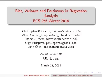
Bias and Parsimony in Regression Analysis ECS 256 W14 Final Project Presentaion Kevin Cosgrove, Wei Fang, Xiaoyun Wang, Zhicheng Yang Department of Computer Science University of California, Davis March 11, 2014

O UTLINE P ROBLEM 1 Bias Of An Approximate Regression Model P ROBLEM 2 a. Parsimony b. Testing On Simulated Data c. Testing On Real Data Sets d. Another PAC Function

P ROBLEM D ESCRIPTION The population regression function is m Y ; X ( t ) = t 0 . 75 t ∈ ( 0 , 1 ) (1) The estimated regression function is ˆ m Y ; X ( t ) = β t t ∈ ( 0 , 1 ) (2) Find the asymptotic bias at t = 0.5.

S OLUTION The key is Eqn.(23.34) ˆ β = ( Q ′ Q ) − 1 Q ′ V   Y 1 Y 2   � � where in this case, V =  , Q = X 1 , X 2 , · · · , X n  .  .   .  Y n plug into Eqn.(23.34), n n ˆ � � X 2 i ) − 1 β = ( X i Y i (3) i = 1 i = 1 As the sample size n goes to infinity, β = E ( XY ) (4) E ( X 2 )

S OLUTION ( CONT .) β = E ( XY ) E ( X 2 ) The population regression function m Y ; X ( t ) = t 0 . 75 t ∈ ( 0 , 1 ) is equivalent to, E ( Y | X = t ) = t 0 . 75 t ∈ ( 0 , 1 ) (5) E ( Y | X ) = X 0 . 75 X ∼ U ( 0 , 1 ) (6) E ( XY ) = E [ E ( XY | X )] = E [ XE ( Y | X )] = E ( X 1 . 75 ) � 1 � 1 1 E ( X 1 . 75 ) = t 1 . 75 f X ( t ) dt = t 1 . 75 dt = 2 . 75 0 0 � 1 � 1 t 2 dt = 1 E ( X 2 ) = t 2 f X ( t ) dt = 3 0 0

S OLUTION ( CONT .) 3 β = 2 . 75 = 1 . 090909091 The bias function is bias ( t ) = E [ ˆ m Y ; X ( t )] − m Y ; X ( t ) (7) = E ( β t ) − t 0 . 75 (8) = 0 . 5 β − t 0 . 75 t ∈ ( 0 , 1 ) (9) At t = 0 . 5 the bias is bias ( t = 0 . 5 ) = − 0 . 04914901

O UTLINE P ROBLEM 1 Bias Of An Approximate Regression Model P ROBLEM 2 a. Parsimony b. Testing On Simulated Data c. Testing On Real Data Sets d. Another PAC Function

P ROBLEM 2 A . P ARSIMONY ◮ Goal: Develop a model selection method that yields parsimony no matter how large the sample data is. ◮ Function Declarations: prsm(y,x,k=0.01,predacc=ar2,crit,printdel=F) ar2(y,x) aiclogit(y,x) compare(y,x,predacc) ◮ In prsm(), predictor variables are deleted in the least "significant" order. ◮ ar2() is a "max" PAC function. ◮ New PAC value is acceptable if > ( 1 − k ) PAC. ◮ aiclogit() is a "min" PAC function. ◮ New PAC value is acceptable if < ( 1 + k ) PAC.

P ROBLEM 2 B . T ESTING O N S IMULATED D ATA T ABLE : Recommended Predictor Set Parsimony Model Sample size Runs Significance Testing k=0.01 k=0.05 1 1 2 3 9 1 2 3 1 2 3 9 100 2 1 2 3 6 7 9 1 2 3 6 7 9 1 2 3 7 3 1 2 3 1 2 3 1 2 3 1 1 2 3 1 2 3 1 2 3 4 1000 2 1 2 3 1 2 3 1 2 3 3 1 2 3 1 2 3 1 2 3 1 1 2 3 1 2 3 1 2 3 4 10000 2 1 2 3 1 2 3 1 2 3 4 9 3 1 2 3 1 2 3 1 2 3 4 1 1 2 3 1 2 3 1 2 3 4 7 100000 2 1 2 3 1 2 3 1 2 3 4 3 1 2 3 1 2 3 1 2 3 4 8

P ROBLEM 2 C . T ESTING O N R EAL D ATA S ETS Data set criteria: ◮ Small n (< 1000), small p (< 10), continuous Y ◮ Data Set #1: Concrete Compressive Strength ◮ Small n (< 1000), small p (< 10), 0-1 Y ◮ Data Set #2: Pima Indians Diabetes ◮ Small n (< 1000), large p (> 15), continuous Y ◮ Data Set #3: Parkinsons ◮ Small n (< 1000), large p (> 15), 0-1 Y ◮ Data Set #4: Ionosphere ◮ Large n (> 5000), small p (< 10), continuous Y ◮ Data Set #5: Wine Quality ◮ Large n (> 5000), small p (< 10), 0-1 Y ◮ Data Set #6: Page Blocks Classification ◮ Large n (> 5000), large p (> 15), continuous Y ◮ Data Set #7: Waveform Database Generator ◮ Large n (> 5000), large p (> 15), 0-1 Y ◮ Data Set #8: EEG Eye State

D ATA S ET #1: C ONCRETE C OMPRESSIVE S TRENGTH ◮ Small n = 1030, small p = 9, continuous Y ◮ This data set consists of 7 concrete mixtures’ component densities, the age since it was poured, and its compressive strength. The densities and the age are the set’s predictor variables (total of 8), and the strength is the response variable. ◮ We chose to use the ar2 PAC function with k = 0.01 and 0.05, as well as significance testing with α = 5%. These tests deleted 3, 3, and 2 predictor variables, respectively. T ABLE : Test Result On Data Set # 1 Parsimony Model Date Set # Significance Testing k=0.01 k=0.05 1 1 2 3 4 8 1 2 3 4 8 1 2 3 4 5 8

D ATA S ET #2: P IMA I NDIANS D IABETES ◮ Small n = 768, small p = 8, 0-1 Y ◮ This data set consists of 8 different medical measures of Pima Indian women over the age of 21, and a boolean class variable. ◮ We chose to use the AIC PAC function with k = 0.01 and 0.05, and significance testing with α = 5%. These tests deleted 4, 7, and 3 predictor variables, respectively. T ABLE : Test Result On Data Set # 2 Parsimony Model Date Set # Significance Testing k=0.01 k=0.05 2 1 2 6 7 2 1 2 3 6 7

D ATA S ET #3: P ARKINSONS ◮ Small n = 197, large p = 23, continuous Y ◮ This data set is composed of 22 medical measures of patients with or without Parkinson’s disease. The predictor varaibles are the results of the medical tests and the response variable is a boolean for the presence of Parkinson’s. ◮ We chose to use the ar2 PAC function with k = 0.01 and 0.05, and significance testing with α = 5%. These tests deleted 11, 15, and 19 predictor variables, respectively. T ABLE : Test Result On Data Set # 3 Parsimony Model Date Set # Significance Testing k=0.01 k=0.05 3 1 3 4 8 9 12 15 1 4 8 19 20 4 17 20 16 17 19 20

D ATA S ET #4: I ONOSPHERE ◮ Small n = 351, large p = 34, 0-1 Y ◮ This data set consists of measurements of electromagnetic tests in the ionosphere and a boolean class value. ◮ The second column for the data set was all zeros. ◮ We chose to use the AIC PAC function with k = 0.01 and 0.05, and significance testing with α = 5%. These tests deleted 15, 24, and 20 predictor variables, respectively. T ABLE : Test Result On Data Set # 4 Parsimony Model Date Set # Significance Testing k=0.01 k=0.05 4 1 4 5 7 8 10 14 1 4 5 7 14 21 26 1 2 4 6 7 8 18 21 22 25 15 17 18 21 22 28 29 33 26 30 33 24 26 28 29 30 33

D ATA S ET #5: W INE Q UALITY ◮ Large n = 4898, small p = 12, continuous Y ◮ This data set is composed of measures of different types of white wine. The response variable is a rating tasting score between 0 and 10, and the 11 predictor variables are various chemical measures. ◮ We chose to use the ar2 PAC function with k = 0.01 and 0.05, and significance testing with α = 5%. These tests deleted 4, 8, and 3 predictor variables, respectively. T ABLE : Test Result On Data Set # 5 Parsimony Model Date Set # Significance Testing k=0.01 k=0.05 5 1 3 4 8 1 3 4 1 2 3 4 5 6 7 8 9

D ATA S ET #6: P AGE B LOCKS C LASSIFICATION ◮ Large n = 5473, small p = 10, 0-1 Y ◮ This data set consists of 11 different measures relating to the amount of black and white space in parts of different text documents. None of the variables are inherently response variables, but we chose the number of white-black transitions to be the response variable for our tests. ◮ We chose to use the AIC PAC function with k = 0.01 and 0.05, and significance testing with α = 5%. These tests deleted 3, 5, and zero predictor variables, respectively. T ABLE : Test Result On Data Set # 6 Parsimony Model Date Set # Significance Testing k=0.01 k=0.05 6 1 2 3 4 5 6 10 1 2 4 5 6 1 2 3 4 5 6 7 8 9 10

D ATA S ET #7: W AVEFORM D ATABASE G ENERATOR ◮ Large n = 5000, large p = 40, continuous Y ◮ This data set is composed of 40 predictor variables which are different measures of waves, about half of which are normalized. The response variable is one of 3 different types of waves. ◮ We chose to use the ar2 PAC function with k = 0.01 and 0.05, and significance testing with α = 5%. These tests deleted 34, 37, and 25 predictor variables, respectively. T ABLE : Test Result On Data Set # 7 Parsimony Model Date Set # Significance Testing k=0.01 k=0.05 7 5 6 10 11 12 13 16 11 12 3 4 5 6 7 9 10 11 12 13 14 15 17 18 19

D ATA S ET #8: EEG E YE S TATE ◮ Large n = 14980, large p = 15, 0-1 Y ◮ This data set consists of 14 measures of an EEG test with the response variable a boolean indicating whether the subject’s eyes were open or closed. ◮ We chose to use the AIC PAC function with k = 0.01 and 0.05, and significance testing with α = 5%. These tests deleted 10, 13, and 1 variables, respectively. T ABLE : Test Result On Data Set # 8 Parsimony Model Date Set # Significance Testing k=0.01 k=0.05 8 1 2 5 6 2 1 2 3 4 5 6 7 9 10 11 12 13 14

P ROBLEM 2 D . A NOTHER PAC F UNCTION ◮ Leave-one-out cross-validation. ◮ PAC value is the proportion of correct classfications. So this is a "max" PAC function. ◮ The PAC function’s running time is linear with the sample size. ◮ Two implementations: ◮ Self-made cross-validation: For each observation in the sample data, we temporarily delete it from training set, and reserve it as the validation set. Perform the training-validation process though every observation, count the number of correct classifications. Return the proportion of correct predictions. ◮ Use R’s cv.glm() function in boot package.