Parsimony Small Parsimony and Search Algorithms Genome 559: - PowerPoint PPT Presentation
Parsimony Small Parsimony and Search Algorithms Genome 559: Introduction to Statistical and Computational Genomics Elhanan Borenstein A quick review The parsimony principle: Find the tree that requires the fewest evolutionary changes!
Parsimony Small Parsimony and Search Algorithms Genome 559: Introduction to Statistical and Computational Genomics Elhanan Borenstein
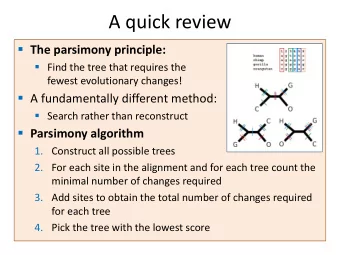
A quick review � The parsimony principle: � Find the tree that requires the fewest evolutionary changes! � A fundamentally different method: � Search rather than reconstruct � Parsimony algorithm 1. Construct all possible trees 2. For each site in the alignment and for each tree count the minimal number of changes required 3. Add sites to obtain the total number of changes required for each tree 4. Pick the tree with the lowest score
A quick review � The parsimony principle: � Find the tree that requires the fewest evolutionary changes! � A fundamentally different method: � Search rather than reconstruct � Parsimony algorithm 1. Construct all possible trees Too many! 2. For each site in the alignment and for each tree count the The small minimal number of changes required parsimony problem 3. Add sites to obtain the total number of changes required for each tree 4. Pick the tree with the lowest score
Large vs. Small Parsimony � We divided the problem of finding the most parsimonious tree into two sub-problems: � Large parsimony: Find the topology which gives best score � Small parsimony : Given a tree topology and the state in all the tips, find the minimal number of changes required � Large parsimony is “NP-hard” � Small parsimony can be solved quickly using Fitch’s algorithm
The Small Parsimony Problem � Input: 1. A tree topology: 2. State assignments for all tips: Human C A C T Chimp T A C T Bonobo A G C C Gorilla A G C A Gibbon G A C T Lemur T A G T human chimp gibbon lemur gorilla bonobo human chimp gibbon lemur gorilla bonobo C T G T A A � Output: The minimal number of changes required: parsimony score ( but in fact, we will also find the most parsimonious assignment for all internal nodes )
Fitch’s algorithm � Execute independently for each character: � Two phases: 1. Bottom-up phase : Determine the set of possible states for each internal node 2. Top-down phase : Pick a state for each internal node 1 2 human chimp gibbon lemur gorilla bonobo C T G T A A
1. Fitch’s algorithm: Bottom-up phase (Determine the set of possible states for each internal node) 1. Initialization: R i = { s i } for all tips 2. Traverse the tree from leaves to root (“post-order”) 3. Determine R i of internal node i with children j , k: if R ∩ R ≠ φ → R ∩ R j k j k R = i otherwise → R ∪ R j k T,A Let s i denote the T state of node i and R i 1 G,T,A the set of possible C,T states of node i G,T human chimp gibbon lemur gorilla bonobo C T G T A A
1. Fitch’s algorithm: Bottom-up phase (Determine the set of possible states for each internal node) 1. Initialization: R i = { s i } 2. Traverse the tree from leaves to root (“post-order“) 3. Determine R i of internal node i with children j , k: if R ∩ R ≠ φ → R ∩ R j k j k R = i otherwise → R ∪ R j k Parsimony-score = T,A # union operations T 1 G,T,A C,T G,T Parsimony-score = 4 human chimp gibbon lemur gorilla bonobo C T G T A A
2. Fitch’s algorithm: Top-down phase (Pick a state for each internal node) 1. Pick arbitrary state in R root to be the state of the root , s root 2. Traverse the tree from root to leaves (“pre-order”) 3. Determine s i of internal node i with parent j : if s ∈ R → s j i j s = i otherwise → arbitrary state ∈ R i T,A T 2 G,T,A C,T G,T Parsimony-score = 4 human chimp gibbon lemur gorilla bonobo C T G T A A
2. Fitch’s algorithm: Top-down phase (Pick a state for each internal node) 1. Pick arbitrary state in R root to be the state of the root ,s root 2. Traverse the tree from root to leaves (“pre-order”) 3. Determine s i of internal node i with parent j : if s ∈ R → s j i j s = i otherwise → arbitrary state ∈ R i A T 2 T T T Parsimony-score = 4 human chimp gibbon lemur gorilla bonobo C T G T A A
And now back to the “big” parsimony problem … How do we find the most parsimonious tree amongst the many possible trees?
Searching tree space � Exhaustive search : Up to 8-10 leaves (10k-2m unrooted trees, 135k-34m rooted) Guaranteed results � Branch-and-bound*: Up to 10-20 leaves Guaranteed results!!! * Branch-and-bound is a clever way of ruling out most trees as they are built, so you can evaluate more trees by exhaustive search. � Heuristic search (e.g. hill-climb) : 20+ leaves May not find correct solution.
Hill-climbing still possible Final tree that best Parsimony tree is here score Accepted related tree Different trees Rejected related tree Starting tree A “greedy” algorithm
Nearest-Neighbor Interchange (NNI) 1. Find a tree with some score. 2. At each internal branch consider the two alternative arrangements of the 4 sub-trees. 3. Keep the tree that has the best score. 4. Repeat. Sub-tree
three (of many) places where NNI can be considered
Hill-climbing with NNI still possible Final tree that best Parsimony tree is here score Accepted NNI tree Different trees Rejected NNI tree Starting tree A “greedy” algorithm
How can we improve this algorithm and increase our chances of finding the optimal tree?
The parsimony algorithm 1) Construct all possible trees or search the space of possible trees using NNI hill-climb 2) For each site in the alignment and for each tree count the minimal number of changes required using Fitch’s algorithm 3) Add all sites up to obtain the total number of changes for each tree 4) Pick the tree with the lowest score or search until no better tree can be found
Phylogenetic trees: Summary Parsimony Trees: Distance Trees: 1)Construct all possible trees or 1)Compute pairwise corrected search the space of possible trees distances. 2)For each site in the alignment and 2)Build tree by sequential clustering for each tree count the minimal algorithm (UPGMA or Neighbor- number of changes required using Joining). Fitch’s algorithm 3)These algorithms don't consider 3)Add all sites up to obtain the total all tree topologies, so they are number of changes for each tree very fast, even for large trees. 4)Pick the tree with the lowest score Maximum-Likelihood Trees: 1)Tree evaluated for likelihood of data given tree. 2)Uses a specific model for evolutionary rates (such as Jukes-Cantor). 3)Like parsimony, must search tree space. 4)Usually most accurate method but slow.
Branch confidence How certain are we that this is the correct tree? Can be reduced to many simpler questions - how certain are we that each branch point is correct? For example, at the circled branch point, how certain are we that the three subtrees have the correct content : subtree1 - QUA025, QUA013 subtree2 - QUA003, QUA024, QUA023 subtree3 - everything else
Bootstrap support Most commonly used branch support test: 1. Randomly sample alignment sites. 2. Use sample to estimate the tree. 3. Repeat many times. (sample with replacement means that a sampled site remains in the source data after each sampling, so that some sites will be sampled more than once)
Bootstrap support For each branch point on the computed tree, count what fraction of the bootstrap trees have the same subtree partitions (regardless of topology within the subtrees). For example at the circled branch point, what fraction of the bootstrap trees have a branch point where the three subtrees include: subtree1 - QUA025, QUA013 subtree2 - QUA003, QUA024, QUA023 subtree3 - everything else This fraction is the bootstrap support for that branch.
Original tree figure with branch supports (here as fractions, also common to give % support) low-confidence branches are marked
Recommend
More recommend
Explore More Topics
Stay informed with curated content and fresh updates.
