Computing parsimony Parsimony treats each site (position in a - PowerPoint PPT Presentation
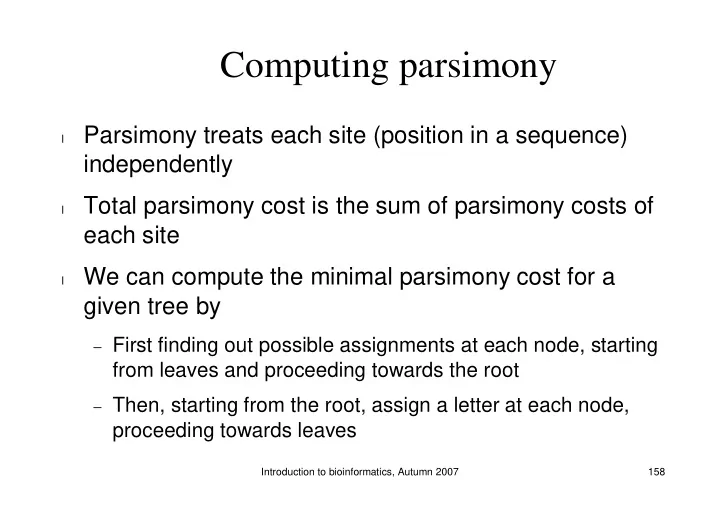
Computing parsimony Parsimony treats each site (position in a sequence) l independently Total parsimony cost is the sum of parsimony costs of l each site We can compute the minimal parsimony cost for a l given tree by First finding out
Computing parsimony Parsimony treats each site (position in a sequence) l independently Total parsimony cost is the sum of parsimony costs of l each site We can compute the minimal parsimony cost for a l given tree by − First finding out possible assignments at each node, starting from leaves and proceeding towards the root − Then, starting from the root, assign a letter at each node, proceeding towards leaves Introduction to bioinformatics, Autumn 2007 158
Labelling tree nodes An unrooted tree with n leaves contains 2n-1 nodes l altogether Assign the following labels to nodes in a rooted tree l − leaf nodes: 1, 2, …, n − internal nodes: n+1, n+2, …, 2n-1 9 − root node: 2n-1 The label of a child node is always l 8 smaller than the label of the 6 7 parent node 1 2 3 4 5 Introduction to bioinformatics, Autumn 2007 159
Parsimony algorithm: first phase Find out possible assignments at every node for each site u l independently. Denote site u in sequence i by s i,u. For i := 1, … , n do F i := {s i,u } % possible assignment s at node i L i := 0 % number of subst it ut ions up t o node i For i := n+1, … , 2n-1 do Let j and k be t he children of node i I f F j � F k = � t hen L i := L j + L k + 1, F i := F j � F k else L i := L j + L k , F i := F j � F k Introduction to bioinformatics, Autumn 2007 160
Parsimony algorithm: first phase Choose u = 3 (for example, in general we do this for all u) F 1 := {T} L 1 := 0 9 F 2 := {A} L 2 := 0 7 F 3 := {C}, L 3 := 0 6 8 F 4 := {T}, L 4 := 0 3 4 5 2 1 F 5 := {T}, L 5 := 0 AA C GT AA T GT AA T TT AC A TT AC T TT Introduction to bioinformatics, Autumn 2007 161
Parsimony algorithm: first phase F 6 := F 3 � F 4 = {C, T} L 6 := L 3 + L 4 + 1 = 1 9 T F 7 := F 5 � F 6 = {T} 7 T L 7 := L 5 + L 6 = 1 6 {C,T} 8 {A, T} F 8 := F 1 � F 2 = {A, T} L 8 := L 1 + L 2 + 1 = 1 3 4 5 2 1 AA C GT AA T GT AA T TT AC A TT AC T TT F 9 := F 7 � F 8 = {T} L 9 := L 7 + L 8 = 2 � Parsimony cost for site 3 is 2 Introduction to bioinformatics, Autumn 2007 162
Parsimony algorithm: second phase Backtrack from the root and assign x � F i at each node l If we assigned y at parent of node i and y � F i , then l assign y Else assign x � F i by random l Introduction to bioinformatics, Autumn 2007 163
Parsimony algorithm: second phase At node 6, the algorithm assigns T because T 9 T was assigned to parent node 7 and T � F 6 . 7 T T is assigned to node 8 6 {C, T } 8 {A, T } for the same reason. 3 4 5 2 1 AA C GT AA T GT AA T TT AC A TT AC T TT The other nodes have only one possible letter to assign Introduction to bioinformatics, Autumn 2007 164
Parsimony algorithm First and second phase are repeated for each site in the sequences, 9 T summing the parsimony costs at each site 7 T 6 T 8 T 3 4 5 2 1 AA C GT AA T GT AA T TT AC A TT AC T TT Introduction to bioinformatics, Autumn 2007 165
Properties of parsimony algorithm Parsimony algorithm requires that the sequences are l of same length − First align the sequences against each other and remove indels − Then compute parsimony for the resulting sequences Is the most parsimonious tree the correct tree? l − Not necessarily but it explains the sequences with least number of substitutions − We can assume that the probability of having fewer mutations is higher than having many mutations Introduction to bioinformatics, Autumn 2007 166
Finding the most parsimonious tree Parsimony algorithm calculates the parsimony cost for l a given tree… …but we still have the problem of finding the tree with l the lowest cost Exhaustive search (enumerating all trees) is in general l impossible More efficient methods exist, for example l − Probabilistic search − Branch and bound Introduction to bioinformatics, Autumn 2007 167
Branch and bound in parsimony We can exploit the fact that adding edges to a tree can l only increase the parsimony cost {C, T} {T} {T} 1 2 3 1 2 AA C GT AA T GT AA T TT AA T GT AA T TT cost 0 cost 1 Introduction to bioinformatics, Autumn 2007 168
Branch and bound in parsimony In parsimony… Branch and bound is a general search strategy Start from a tree with 1 l where sequence Each solution is potentially Add a sequence to the tree l l generated and calculate parsimony cost Track is kept of the best l solution found If the tree is complete, check l if found the best tree so far If a partial solution cannot l achieve better score, we If tree is not complete and l abandon the current search cost exceeds best tree cost, path do not continue adding edges to this tree Introduction to bioinformatics, Autumn 2007 169
Branch and bound graphically … … 4 3 1 2 Partial tree, no best complete tree constructed yet Complete tree: calculate parsimony cost and store Partial tree, cost exceeds the cost of the best tree this far Introduction to bioinformatics, Autumn 2007 170
Distance methods The parsimony method works on sequence (character l string) data We can also build phylogenetic trees in a more l general setting Distance methods work on a set of pairwise distances l d ij for the data Distances can be obtained from phenotypes as well as l from genotypes (sequences) Introduction to bioinformatics, Autumn 2007 171
Distances in a phylogenetic tree Distance matrix D = (d ij ) l gives pairwise distances for leaves of the phylogenetic 7 tree 6 8 In addition, the phylogenetic l tree will now specify 1 2 3 4 5 distances between leaves Distance d ij states how and internal nodes far apart species i and j − Denote these with d ij as well are evolutionary (e.g., number of mismatches in aligned sequences) Introduction to bioinformatics, Autumn 2007 172
Distances in evolutionary context Distances d ij in evolutionary context satisfy the l following conditions − Symmetry: d ij = d ji for each i, j − Distinguishability: d ij � 0 if and only if i � j − Triangle inequality: d ij � d ik + d kj for each i, j, k Distances satisfying these conditions are called metric l In addition, evolutionary mechanisms may impose l additional constraints on the distances � additive and ultrametric distances Introduction to bioinformatics, Autumn 2007 173
Additive trees A tree is called additive , if the distance between any l pair of leaves (i, j) is the sum of the distances between the leaves and the first node k that they share in the tree d ij = d ik + d jk ”Follow the path from the leaf i to the leaf j to find the l exact distance d ij between the leaves.” Introduction to bioinformatics, Autumn 2007 174
Additive trees: example A B C D A C A 0 2 4 4 1 1 2 B 2 0 4 4 1 1 C 4 4 0 2 B D D 4 4 2 0 Introduction to bioinformatics, Autumn 2007 175
Ultrametric trees A rooted additive tree is called a ultrametric tree , if the l distances between any two leaves i and j, and their common ancestor k are equal d ik = d jk Edge length d ij corresponds to the time elapsed since l divergence of i and j from the common parent In other words, edge lengths are measured by a l molecular clock with a constant rate Introduction to bioinformatics, Autumn 2007 176
Identifying ultrametric data We can identify distances to be ultrametric by the l three-point condition: D corresponds to an ultrametric tree if and only if for any three species i, j and k, the distances satisfy d ij � max(d ik , d kj ) If we find out that the data is ultrametric, we can utilise l a simple algorithm to find the corresponding tree Introduction to bioinformatics, Autumn 2007 177
Ultrametric trees 9 8 Time 7 6 Observation time 5 4 3 2 1 Introduction to bioinformatics, Autumn 2007 178
Ultrametric trees 9 d 8,9 Only vertical segments of the tree have correspondence to 8 some distance d ij : Time Horizontal segments act as 7 connectors. 6 Observation time 5 4 3 2 1 Introduction to bioinformatics, Autumn 2007 179
Ultrametric trees 9 d ik = d jk for any two leaves i, j and any ancestor k of i and j 8 Time 7 6 Observation time 5 4 3 2 1 Introduction to bioinformatics, Autumn 2007 180
Ultrametric trees 9 Three-point condition: there exists no leaf leaf i, j for which d ij > max(d ik , d jk ) 8 Time for some leaf leaf k. 7 6 Observation time 5 4 3 2 1 Introduction to bioinformatics, Autumn 2007 181
UPGMA algorithm UPGMA (unweighted pair group method using l arithmetic averages) constructs a phylogenetic tree via clustering The algorithm works by at the same time l − Merging two clusters − Creating a new node on the tree The tree is built from leaves towards the root l UPGMA produces a ultrametric tree l Introduction to bioinformatics, Autumn 2007 182
Cluster distances Let distance d ij between clusters C i and C j be l that is, the average distance between points (species) in the cluster. Introduction to bioinformatics, Autumn 2007 183
Recommend
More recommend
Explore More Topics
Stay informed with curated content and fresh updates.
