Bayesian Reasoning Todays Class Probability theory Posteriors and - PDF document

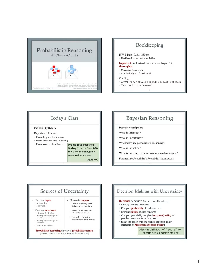
Bookkeeping Probabilistic Reasoning • HW 2 Due 10/3, 11:59pm AI Class 9 (Ch. 13) • Blackboard assignment open Friday • Important : understand the math in Chapter 13 thoroughly • Underpins future work • Also basically all of modern AI A B • Grading • A = 92-100, A- = 90-92, B is 82-87, B- is 80-82, B+ is 88-89, etc Based on slides by Dr. Marie desJardin. Some material also adapted from slides by Dr. • These may be revised downward. Matuszek @ Villanova University, which are based in part on www.csc.calpoly.edu/ ~fkurfess/Courses/CSC-481/W02/Slides/Uncertainty.ppt and www.cs.umbc.edu/ Cynthia Matuszek – CMSC 671 courses/graduate/671/fall05/slides/c18_prob.ppt 2 Bayesian Reasoning Today’s Class • Probability theory • Posteriors and priors • What is inference? • Bayesian inference • From the joint distribution • What is uncertainty? • Using independence/factoring • When/why use probabilistic reasoning? • From sources of evidence Probabilistic inference: finding posterior probability • What is induction? for a proposition, given • What is the probability of two independent events? observed evidence. • Frequentist/objectivist/subjectivist assumptions – R&N 490 3 4 Sources of Uncertainty Decision Making with Uncertainty • Uncertain inputs • Uncertain outputs • Rational behavior: f or each possible action, • Missing data • Default reasoning (even • Identify possible outcomes • Noisy data deduction) is uncertain • Compute probability of each outcome • Uncertain knowledge • Abduction & induction • Compute utility of each outcome inherently uncertain • >1 cause à >1 effect • Compute probability-weighted (expected) utility of • Incomplete knowledge of • Incomplete deductive conditions or effects possible outcomes for each action inference can be uncertain • Incomplete knowledge of • Select the action with the highest expected utility causality (principle of Maximum Expected Utility ) • Probabilistic effects Also the definition of “rational” for Probabilistic reasoning only gives probabilistic results deterministic decision-making. (summarizes uncertainty from various sources) 5 6 1

Probability Basic Probability A B • World: The complete set of states • Each P is a non-negative value in [0,1] • Total probability of the sample space is 1 • Event: Something that happens • For mutually exclusive events , the probability for • Sample Space: All the things (outcomes) that at least one of them is the sum of their individual could happen in some set of circumstances probabilities • Pull 2 squares from envelope A: what is the sample space? • Experimental probability • How about envelope B? • Based on frequency of past events • Probability P ( x ) : likelihood of event x occurring • Subjective probability • Pull a few more squares. • Based on expert assessment • How many of each did you get from A? From B? 8 CSC 4510.9010 Spring 2015. Paula Matuszek Why Probabilities Anyway? Compound Probabilities a a ∧ b b 3 simple axioms à all rules of probability theory* • Describe independent events • Do not affect each other in any way 1. All probabilities are between 0 and 1. • 0 ≤ P ( a ) ≤ 1 • Joint probability of two independent events A and B 2. Valid propositions (tautologies) have probability 1, P (A ∩ B) = P (A) * P (B) What do these say? and unsatisfiable propositions have probability 0. • Union probability of two independent events A and B • P ( true ) = 1 P (A ∪ B) = P (A) + P(B) - P(A ∩ B) • P ( false ) = 0 = P(A) + P(B) - (P(A) * P(B)) a a ∧ b b 3. The probability of a disjunction is: Pull two squares from envelope A. What is the • P ( a ∨ b ) = P ( a ) + P ( b ) – P ( a ∧ b ) probability that they are BOTH red? *Kolmogorov – https://en.wikipedia.org/wiki/Andrey_Kolmogorov De Finetti, Cox, and Carnap have also provided compelling arguments for these axioms 10 CSC 4510.9010 Spring 2015. Paula Matuszek Probability Theory Probability Theory: Definitions • Random variables: • Alarm ( A ), Burglary ( B ), • Conditional • Product rule : Earthquake ( E ) probability • Domain: possible values • P ( a ∧ b ) = P ( a | b ) P ( b ) • Boolean, discrete, continuous • Atomic event: • Probability of effect given cause(s) • A= true ∧ B= true ∧ E= false : • Marginalizing : • Complete specification of a state • alarm ∧ burglary ∧ ¬earthquake • Computing conditional • Finding distribution over • Prior probability: • P ( B ) = 0.1 probability: a subset of variables • Degree of belief without • P ( A , B ) = • P ( a | b ) = � • P ( B ) = Σ a P ( B , a ) any new evidence P ( a ∧ b ) / P ( b ) • P ( B ) = Σ a P ( B | a ) P ( a ) • Joint probability: alarm ¬ alarm ( conditioning ) • P ( b ): normalizing • Matrix of combined burglary 0.09 0.01 constant probabilities of a set of ¬ burglary 0.1 0.8 variables 11 12 2

Try It... Probability Theory (cont.) • Cond’l probability • Cond’l probability • P ( A | B ) = ? • P ( A | B ) = 0.9 � • P(effect, cause[s]) • P(effect, cause[s]) • P ( B | A ) = ? P ( B | A ) = 0.47 • P ( a | b ) = P ( a ∧ b ) / P ( b ) • P ( a | b ) = P ( a ∧ b ) / P ( b ) • P ( B ∧ A ) = ? • P ( B | A ) = P ( B ∧ A ) / P ( A ) = � • P ( b ): normalizing • Here, P ( b ): normalizing 0.09 / 0.19 = 0.47 • P ( A ) = ? constant constant ( α ) • P ( B ∧ A ) = P ( B | A ) P ( A ) = � • Product rule : • Product rule : 0.47 × 0.19 = 0.09 • P ( a ∧ b ) = P ( a | b ) P ( b ) • P ( a ∧ b ) = P ( a | b ) P ( b ) alarm ¬ alarm • Marginalizing : • Marginalizing : burglary 0.09 0.01 • P ( A ) = � P ( A ∧ B ) + P ( A ∧ ¬ B ) = � • P ( B ) = Σ a P ( B , a ) ¬ burglary 0.1 0.8 • P ( B ) = Σ a P ( B , a ) 0.09 + 0.1 = 0.19 • P ( B ) = Σ a P ( B | a ) P ( a ) • P ( B ) = Σ a P ( B | a ) P ( a ) ( conditioning ) ( conditioning ) 13 14 Example: Inference from the Joint Exercise: Inference from the Joint • Queries: what is… • P ( B | A ) = α P ( B , A ) � A ¬A • The prior probability of smart ? = α [ P ( B , A , E ) + P ( B , A , ¬ E ) � E ¬E E ¬E • The prior probability of study ? = α [(.01, .01) + (.08, .09)] � B 0.01 0.08 0.001 0.009 • The conditional probability of prepared , given study and smart ? = α [(.09, .1)] ¬B 0.01 0.09 0.01 0.79 • Save these answers for later! J • Since � P ( B | A ) + P (¬ B | A ) = 1, α = 1 / (0.09 + 0.1) = 5.26 � smart ¬ smart (i.e., P ( A ) = 1/ α = 0.19) P ( smart ∧ study ∧ prep ) study ¬ study study ¬ study • P ( B | A ) = 0.09 * 5.26 = 0.474 quizlet: how can prepared .432 .16 .084 .008 you verify this? • P (¬ B | A ) = 0.1 * 5.26 = 0.526 ¬ prepared .048 .16 .036 .072 15 16 Independence: ⫫ Independence Example • Independent: Two sets of propositions that do • { moon-phase , light-level } ⫫ { burglary , alarm , earthquake } not affect each others’ probabilities • But maybe burglaries increase in low light • But, if we know the light level, moon-phase ⫫ burglary • Easy to calculate joint and conditional probability • Once we’re burglarized, light level doesn’t affect whether of independence: the alarm goes off; { light-level } ⫫ { alarm } ( A , B ) ó P ( A ∧ B ) = P ( A ) P ( B ) or P ( A | B ) = P ( A ) • We need: • Examples: 1. A more complex notion of independence A ⫫ B ⫫ E = f A ⫫ B ⫫ E = ? A = alarm M = moon phase 2. Methods for reasoning about these kinds of (common) relationships B = burglary L = light level M ⫫ L = f M ⫫ L = ? E = earthquake A ⫫ M = t A ⫫ M = ? 17 18 3