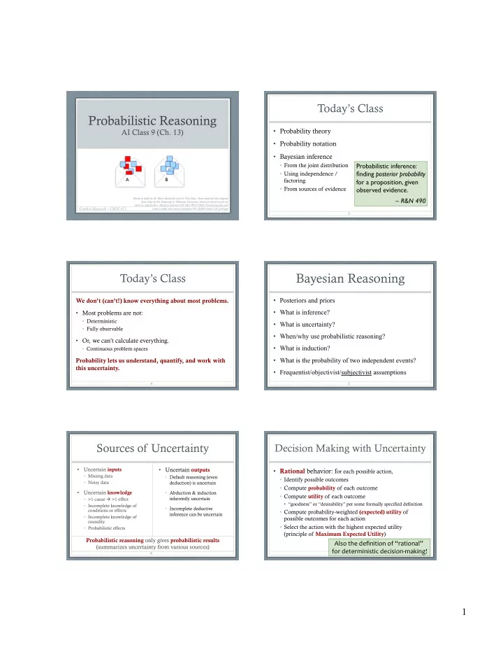
Bayesian Reasoning Todays Class Posteriors and priors We dont - PDF document

Today’s Class Probabilistic Reasoning • Probability theory AI Class 9 (Ch. 13) • Probability notation • Bayesian inference • From the joint distribution Probabilistic inference: • Using independence / finding posterior probability A B factoring for a proposition, given • From sources of evidence observed evidence. Based on slides by Dr. Marie desJardin and Dr. Tim Oates. Some material also adapted – R&N 490 from slides by Dr. Matuszek @ Villanova University, which are based in part on www.csc.calpoly.edu/~fkurfess/Courses/CSC-481/W02/Slides/Uncertainty.ppt and Cynthia Matuszek – CMSC 671 www.cs.umbc.edu/courses/graduate/671/fall05/slides/c18_prob.ppt 3 Bayesian Reasoning Today’s Class • Posteriors and priors We don’t (can’t!) know everything about most problems. • What is inference? • Most problems are not: • Deterministic • What is uncertainty? • Fully observable • When/why use probabilistic reasoning? • Or, we can’t calculate everything. • What is induction? • Continuous problem spaces • What is the probability of two independent events? Probability lets us understand, quantify, and work with this uncertainty. • Frequentist/objectivist/subjectivist assumptions 4 5 Sources of Uncertainty Decision Making with Uncertainty • Uncertain inputs • Uncertain outputs • Rational behavior: f or each possible action, • Missing data • Default reasoning (even • Identify possible outcomes • Noisy data deduction) is uncertain • Compute probability of each outcome • Uncertain knowledge • Abduction & induction • Compute utility of each outcome inherently uncertain • >1 cause à >1 effect • “goodness” or “desirability” per some formally specified definition • Incomplete knowledge of • Incomplete deductive conditions or effects • Compute probability-weighted (expected) utility of inference can be uncertain • Incomplete knowledge of possible outcomes for each action causality • Select the action with the highest expected utility • Probabilistic effects (principle of Maximum Expected Utility ) Probabilistic reasoning only gives probabilistic results Also the definition of “rational” (summarizes uncertainty from various sources) for deterministic decision-making! 6 7 1

Probability Basic Probability A B • World: The complete set of possible states • Each P is a non-negative value in [0,1] • P({1,1}) = 1/36 • Random variables: Problem aspects that take a value • “The number of blue squares we are holding,” B • Total probability of the sample space is 1 • “The combined value of two dice we rolled,” C • P({1,1}) + P({1,2}) + P({1,3}) + … + P({6,6}) = 1 • Event: Something that happens • For mutually exclusive events, the probability for at least one of them is the sum of their individual probabilities • Sample Space: All the things (outcomes) that could • P(sunny) ∨ P(cloudy) = P(sunny) + P(cloudy) happen in some set of circumstances • Pull 2 squares from envelope A: what is the sample space? • Experimental probability: Based on frequency of past events • How about envelope B? • Subjective probability: Based on expert assessment • World, redux: A complete assignment of values to variables 9 commons.wikimedia.org/wiki/File:2-Dice-Icon.svg CSC 4510.9010 Spring 2015. Paula Matuszek Why Probabilities Anyway? Compound Probabilities a a ∧ b b 3 simple axioms à all rules of probability theory* • Describe independent events • Do not affect each other in any way 1. All probabilities are between 0 and 1. • 0 ≤ P ( a ) ≤ 1 • Joint probability of two independent events A and B 2. Valid propositions (tautologies) have probability 1, P (A ∩ B) = P (A) * P (B) What do these say? and unsatisfiable propositions have probability 0. • Union probability of two independent events A and B • P ( true ) = 1 P (A ∪ B) = P (A) + P(B) - P(A ∩ B) • P ( false ) = 0 = P(A) + P(B) - (P(A) * P(B)) a a ∧ b b 3. The probability of a disjunction is: Pull two squares from envelope A. What is the • P ( a ∨ b ) = P ( a ) + P ( b ) – P ( a ∧ b ) probability that they are BOTH red? *Kolmogorov – en.wikipedia.org/wiki/Andrey_Kolmogorov De Finetti, Cox, and Carnap have also provided compelling arguments for these axioms 11 CSC 4510.9010 Spring 2015. Paula Matuszek Probability Theory Probability Distributions • Random variables: • Alarm ( A ), Burglary ( B ), • A distribution is the probabilities of all possible Earthquake ( E ) • Domain: possible values values of a random variable • Boolean, discrete, continuous • Atomic event: • Ex: weather can be sunny, rainy, cloudy, or snowy • A= true ∧ B= true ∧ E= false : • Complete specification of • P(Weather = sun) = 0.6 a state • alarm ∧ burglary ∧ ¬earthquake • P(Weather = rain) = 0.1 • Prior probability: • P( B ) = 0.1 • P(Weather = cloud) = 0.29 • Degree of belief without • P( A , B ) = any new evidence • P(Weather = snow) = 0.01 • Joint probability: • P (Weather) = <0.6, 0.1, 0.29, 0.01> ß shortcut alarm ¬ alarm • Matrix of combined burglary 0.09 0.01 • P (Weather) : probability distribution on Weather probabilities of a set of ¬ burglary 0.1 0.8 variables, P( A | B ) 12 13 2

Probability Theory: Definitions Probability Theory: Definitions • Conditional probability: Probability of some effect • Product rule : given that we know cause(s) • P( a ∧ b ) = P( a | b ) P( b ) • Example: P( alarm | burglary ) • Marginalizing (summing out): • (Technically, we only know b is true, not causal, but…) • Finding distribution over one or a subset of variables • Computing it: • Marginal probability of B summed over all alarm states: P( a ∧ b ) • P( B ) = Σ a P( B , a ) • P( a | b ) = P( b ) • Conditioning over a subset of variables: • P( b ) : normalizing constant • P( B ) = Σ a P( B | a ) P( a ) • (Later we’ll call this alpha) 14 15 alarm ¬ alarm Try It... Example: Inference from the Joint burglary 0.09 0.01 ¬ burglary 0.1 0.8 • Cond’l probability • P ( A | B ) = 0.9 • P ( B | A ) = α P ( B , A ) � A ¬A • P(effect, cause[s]) = α [ P ( B , A , E ) + P ( B , A , ¬ E ) � E ¬E E ¬E • P ( B | A ) = 0.47 • P ( a | b ) = P ( a ∧ b ) / P ( b ) = α [(.01, .01) + (.08, .09)] � B 0.01 0.08 0.001 0.009 • P ( B | A ) = P ( B ∧ A ) / P ( A ) = � • P ( b ): normalizing = α [(.09, .1)] ¬B 0.01 0.09 0.01 0.79 constant (1/ α ) 0.09 / 0.19 = 0.47 • Since � • Product rule : • P ( B ∧ A ) = 0.09 P ( B | A ) + P (¬ B | A ) = 1, α = 1 / (0.09 + 0.1) = 5.26 � • P ( a ∧ b ) = P ( a | b ) P ( b ) • P ( B | A ) P ( A ) = � (i.e., P ( A ) = 1/ α = 0.19) • Marginalizing : 0.47 × 0.19 = 0.09 • P ( B | A ) = 0.09 * 5.26 = 0.474 • P ( B ) = Σ a P ( B , a ) • P ( A ) = 0.19 • P (¬ B | A ) = 0.1 * 5.26 = 0.526 • P ( B ) = Σ a P ( B | a ) P ( a ) • P ( A ∧ B ) + P ( A ∧ ¬ B ) = � ( conditioning ) 0.09 + 0.1 = 0.19 16 17 Exercise: Exercise: Inference from the Joint Inference from the joint smart ¬ smart • Queries: what is… P ( smart ∧ study ∧ prep ) ≈ study ¬ study study ¬ study • The prior probability (knowing nothing else) of smart ? • The prior probability of study ? prepared .432 .16 .084 .008 • The conditional probability of prepared , given study and ¬ prepared .048 .16 .036 .072 smart ? Queries: smart ¬ smart P ( smart ∧ • What is the prior probability of smart ? study ∧ prep ) study ¬ study study ¬ study • What is the prior probability of study ? • What is the conditional probability of prepared , given study prepared .432 .16 .084 .008 and smart ? ¬ prepared .048 .16 .036 .072 P( smart ) = .432 + .16 + .048 + .16 = 0.8 18 19 3