Bayesian Latent Variable Modelling of Longitudinal Family Data for - PowerPoint PPT Presentation

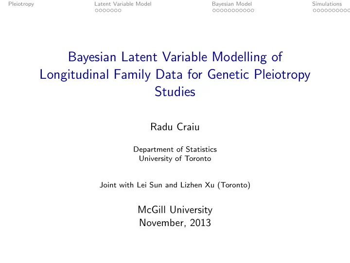
Pleiotropy Latent Variable Model Bayesian Model Simulations Bayesian Latent Variable Modelling of Longitudinal Family Data for Genetic Pleiotropy Studies Radu Craiu Department of Statistics University of Toronto Joint with Lei Sun and Lizhen Xu (Toronto) McGill University November, 2013

Pleiotropy Latent Variable Model Bayesian Model Simulations Outline Pleiotropy Latent Variable Model Data and Statistical Model Statistical Complications Bayesian Model Computational Complications A Parameter Expanded Model for Added Efficiency Variable Selection Simulations Simulation Study Application: GAW 18 Application: Type 1 Diabetes

Pleiotropy Latent Variable Model Bayesian Model Simulations Pleiotropy ◮ For many complex human diseases, the trait of interest (”state of disease”) is not directly observable (e.g. diabetes, hypertension, cardiovascular disease). ◮ Instead we observe a set of surrogate phenotypes (physical manifestations of the disease) which may be continuous or discrete. ◮ These response variables (phenotypes or outcomes) are mutually correlated as they measure the underlying trait from different perspectives. ◮ In order to increase statistical efficiency, it is desirable to model these outcomes jointly. ◮ Many studies also involve repeated measures over time in samples that include families/clusters ⇒ complex dependence structures in the data. ◮ We are considering here continuous and binary phenotypes.

Pleiotropy Latent Variable Model Bayesian Model Simulations The Data and Model ◮ Let Y cit = ( Y c cit T , Y b cit T ) T be the J × 1 vector of responses (e.g. phenotypes) measured at the t th time on the i th individual from the c th family(or cluster) for c = 1 , 2 , ..., C , i = 1 , 2 , ..., N c , t = 1 , 2 , ..., B , and j = 1 , 2 , ..., J , where C denotes the total number of families, N c is the number of individuals within the c th family, B is the total number of repeated measurements and J is the total number of responses. ◮ The dependence patterns are approximated via random effects. ◮ The trait of interest is included as a latent variable U cit in the model.

Pleiotropy Latent Variable Model Bayesian Model Simulations Illustration of the Data Structure W 11 W12 serial dependence Y Y Y Y Y Y 111 112 11J 121 122 12J serial U dependence U 11 12 t 1 t time 0 2 X11 X12 serial Cluster dependence dependence Y 211 Y Y Y Y Y 212 21J 221 222 22J serial dependence U U 21 22 t t 2 time 0 1 X21 X 22

Pleiotropy Latent Variable Model Bayesian Model Simulations The Statistical Model ◮ The latent variable model U cit = X T cit α + Z T cit a c + Q T cit d ci + ǫ cit , (1) iid ∼ N (0 , ψ 2 ). where ǫ cit ◮ d ci ∈ R q 2 × 1 represents the subject-specific random effects. ◮ a c are cluster-specific random effects. iid iid ◮ a c ∼ N q 1 (0 , Σ A ), d ci ∼ N q 2 (0 , Σ D ) and all random effects are independent of the ǫ cit . ◮ We are particularly interested in the regression coefficient for the SNP’s genotype. ◮ Pleiotropy is detected if the SNP’s genotype effect on U is statistically significant.

Pleiotropy Latent Variable Model Bayesian Model Simulations The Statistical Model ◮ The continuous response model y c citj = β 0 j + b cij + W T cit β j + λ j U cit + e citj , (2) iid ∼ N (0 , σ 2 where e citj j ), W cit is a p 1 -dimensional vector of direct effect covariates. ◮ The λ ’s are the factor loadings that allow different contributions of the latent variable to each phenotype. ◮ The random component b cij captures the family-specific within-subject correlations over time. We assume iid ∼ N (0 , τ 2 b cij j ), and e citj and b cij are mutually independent for c = 1 , ..., C , i = 1 , ..., N c , t = 1 , ..., B and j = 1 , ..., J .

Pleiotropy Latent Variable Model Bayesian Model Simulations Statistical Complications - Identifiability ◮ If K ∈ R then cit β j + λ j K − 1 KU cit + b cij + e citj , y c citj = β 0 j + W T (3) ◮ Without any restriction on λ or the variance of U cit , an infinite number of equivalent models can be created. ◮ We assume that: ◮ The variance of U cit is equal to 1 and that λ j is non-negative. ◮ The direct-effect covariates ( W cit ) and the indirect-effect covariates ( X cit , Z cit , Q cit ) are distinct.

Pleiotropy Latent Variable Model Bayesian Model Simulations Statistical Complications - Effect of Ignoring Cluster Correlation ◮ Individuals from the same family are genetically related resulting in correlation between their latent disease status. ◮ If familial dependence is ignored inference is biased. ◮ Consider the case of continuous only phenotypes and no repeated measurements.

Pleiotropy Latent Variable Model Bayesian Model Simulations Statistical Complications - Effect of Ignoring Cluster Correlation ◮ Model 1 (correct): y cij = β 0 j + W T ci β j + λ j U ci + e cij , and U ci = X T ci α + Z T ci a c + ǫ ci , where e cij ∼ N (0 , σ 2 j ) and ǫ ci ∼ N (0 , 1), λ j > 0 and a c ∼ N (0 , Σ A ). ◮ Model 2 (misspecified): h β j + � λ j � � y hj = β 0 j + W T U h = X T U h + e hj , and h � α + ǫ h . ◮ We can show that � λ 2 j = ( Z T ci Σ A Z ci + 1) λ 2 j and α = λ j 1 � α = � α < α. � λ j ( Z T ci Σ A Z ci + 1)

Pleiotropy Latent Variable Model Bayesian Model Simulations Bayesian Model ◮ We consider a Bayesian framework for inference. ◮ If conditional conjugate priors are defined for the model parameters Θ , then a standard Gibbs (SG) sampler can be used to analyze the posterior distribution. ◮ The implementation requires introducing the random effects as latent variables/missing data. The set of all latent variables is denoted Ω.

Pleiotropy Latent Variable Model Bayesian Model Simulations Computational Complications: Torpid Mixing ◮ Due to high dependence between the components of the Markov chain corresponding to the parameter vector Θ and the latent data vector Ω, we observe a very slow mixing of the chain. ◮ For instance, a small variance τ 2 j leads to small random effects b cij and vice versa. Similar patterns develop between the factor loadings λ j and the latent variable U . ◮ These lead to computational inefficiency.

Pleiotropy Latent Variable Model Bayesian Model Simulations Parameter Expansion for Increased Computational Efficiency ◮ Parameter Expansion/Auxiliary Variable methods have a long tradition in MCMC (Besag and Green, JRSSB ’93; Higdon, JASA ’98; Liu and Wu, JASA ’99; van Dyk and Meng, JCGS ’01) ◮ These methods aim at eliminating ”bottlenecks” in simulation experiments by expanding the parameter space or by introducing ”missing” data/latent variables in the model. ◮ However, the parameter expansion guidelines need to be modified/adapted for each model.

Pleiotropy Latent Variable Model Bayesian Model Simulations A Parameter Expanded Model - Continuous Outcomes ◮ Original model is y c citj = β 0 j + b cij + W T cit β j + λ j U cit + e citj , U cit = X T cit α + Z T cit a c + Q T cit d ci + ǫ cit ,

Pleiotropy Latent Variable Model Bayesian Model Simulations A Parameter Expanded Model - Continuous Outcomes ◮ Introduce auxiliary parameters { ξ j : 1 ≤ j ≤ J } and ψ and reparametrise the model. ◮ Transformed model: β 0 j b cij U cit y c + W T citj = ξ j + ξ j cit β j + ψλ j + e citj , ξ j ξ j ψ U cit α a c d ci ψ + ǫ cit = X T ψ + Z T ψ + Q T ψ , cit cit cit ψ

Pleiotropy Latent Variable Model Bayesian Model Simulations A Parameter Expanded Model - Continuous Outcomes ◮ Transformed model: y c citj = ξ j b ∗ cij + W T cit β j + λ ∗ j U ∗ cit + e citj , cit α ∗ + Z T U ∗ cit = X T cit a ∗ c + Q T cit d ∗ ci + ǫ ∗ cit .

Pleiotropy Latent Variable Model Bayesian Model Simulations A Parameter Expanded Model - Continuous Outcomes iid iid ◮ b ∗ cij ∼ N ( β ∗ 0 j , τ ∗ 2 j ), a ∗ ∼ N q 1 (0 , Σ ∗ a ), d ∗ ∼ N q 2 (0 , Σ ∗ d ), and c ci iid ǫ ∗ ∼ N (0 , ψ 2 ). cit ◮ The conditional conjugate priors assigned to θ ∗ = ( α ∗ , λ ∗ . . . , ψ ) impose particular priors on θ = ( α, λ, . . . ). ◮ The parametrization is redundant and the algorithm is not efficient on the expanded state space, but it gains efficiency for the original set of parameters! ◮ The original parameters are recovered using α = α ∗ /ψ, U cit = U ∗ Σ A = Σ ∗ A /ψ 2 , Σ D = Σ ∗ D /ψ 2 , cit /ψ, λ j = λ ∗ β j 0 = β ∗ τ 2 j = ξ 2 j τ ∗ 2 j ψ, j 0 ξ j , j , for all 1 ≤ j ≤ J .

Pleiotropy Latent Variable Model Bayesian Model Simulations A Parameter Expanded Model - Mixed Outcomes ◮ When the traits are mixed denote { y c citj : 1 ≤ j ≤ J 1 } the continuous outcomes and { y b citj : J 1 + 1 ≤ j ≤ J } the binary ones. ◮ The probit model is expanded using the latent variables � y b citj so that y b y b citj = 1 (0 , ∞ ) ( � citj ). ◮ The continuous response models are expanded as before.

Pleiotropy Latent Variable Model Bayesian Model Simulations A Parameter Expanded Model - Mixed Outcomes ◮ Define � y b citj such that y b y b citj = 1 (0 , ∞ ) ( � citj ) ◮ Start with the usual latent model for probit regression y b citj = β 0 j + b cij + W T cit β j + λ j U cit + ǫ � ◮ Use auxiliary parameters { γ j : J 1 + 1 ≤ j ≤ J } β 0 j b cij y b + W T γ j � citj = γ j ξ j + γ j ξ j cit γ j β j + γ j λ j U cit + γ j ǫ ξ j ξ j