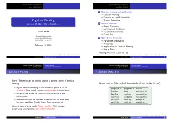
Bayes Classifier (slides borrowed from Tom Mitchell, Barnabs Pczos - PowerPoint PPT Presentation

CSCI 4520 - Introduction to Machine Learning Mehdi Allahyari Georgia Southern University Bayes Classifier (slides borrowed from Tom Mitchell, Barnabás Póczos & Aarti Singh 1

Joint Distribution: sounds like the solution to learning F: X ! Y, or P(Y | X). Main problem: learning P(Y|X) can require more data than we have consider learning Joint Dist. with 100 attributes # of rows in this table? # of people on earth? fraction of rows with 0 training examples? 2

What to do? 1. Be smart about how we estimate probabilities from sparse data – maximum likelihood estimates – maximum a posteriori estimates 2. Be smart about how to represent joint distributions – Bayes networks, graphical models 3

1. Be smart about how we estimate probabilities 4

Principles for Estimating Probabilities Principle 1 (maximum likelihood): • choose parameters θ that maximize P(data | θ ) Principle 2 (maximum a posteriori prob.): • choose parameters θ that maximize P( θ | data) = P(data | θ ) P( θ ) P(data) 5

Two Principles for Estimating Parameters • Maximum Likelihood Estimate (MLE): choose θ that maximizes probability of observed data • Maximum a Posteriori (MAP) estimate: choose θ that is most probable given prior probability and the data 6

Some terminology • Likelihood function: P(data | θ ) • Prior: P( θ ) • Posterior: P( θ | data) • Conjugate prior: P( θ ) is the conjugate prior for likelihood function P(data | θ ) if the forms of P( θ ) and P( θ | data) are the same. 7

You should know Probability basics § random variables, events, sample space, conditional probs, … § independence of random variables § Bayes rule § Joint probability distributions § calculating probabilities from the joint distribution § Point estimation § maximum likelihood estimates § maximum a posteriori estimates § distributions – binomial, Beta, Dirichlet, … § 8

Let’s learn classifiers by learning P(Y|X) Consider Y=Wealth, X=<Gender, HoursWorked> Gender HrsWorked P(rich | G,HW) P(poor | G,HW) F <40.5 .09 .91 F >40.5 .21 .79 M <40.5 .23 .77 M >40.5 .38 .62 9

How many parameters must we estimate? How many parameters must we estimate? Suppose X =<X 1 , … X n > where X i and Y are boolean RV � s To estimate P(Y| X 1 , X 2 , … X n ) If we have 30 boolean X i � s: P(Y | X 1 , X 2 , … X 30 ) 10

Chain Rule & Bayes Rule Chain rule: Bayes rule: Which is shorthand for: Equivalently: 11

Bayesian Learning Use Bayes rule: § § Or equivalently: posterior prior likelihood 12

The Naïve Bayes Classifier 13 13

Can we reduce parameters using Bayes Rule? Suppose X =<X 1 ,… X n > � s where X i and Y are boolean RV’s Y d rows To estimate P(Y| X 1 , X 2 , … X n ) (2 n -1) 2 2 30 ≅ 1 Billion If we have 30 X i ’s instead of 2: P(Y| X 1 , X 2 , … X 30 ) 14

Naïve Bayes Assumption Naïve Bayes assumption: Features X 1 and X 2 are conditionally independent given the class label Y: More generally: 15

Conditional Independence Definition: X is conditionally independent of Y given Z, if the probability distribution governing X is independent of the value of Y, given the value of Z Which we often write E.g., 16

Naïve Bayes Assumption Naïve Bayes uses assumption that the X i are conditionally independent, given Y. Given this assumption, then: in general: How many parameters to describe P(X 1 …X n |Y) ? P(Y) ? 2 (2 n – 1) + 1 Without conditional indep assumption? 2n + 1 With conditional indep assumption? 17

Application of Bayes Rule 18

AIDS test (Bayes rule) Data § Approximately 0.1% are infected § Test detects all infections § Test reports positive for 1% healthy people Probability of having AIDS if test is positive: Only 9%!... 19

Improving the diagnosis Use a weaker follow-up test! § Approximately 0.1% are infected § Test 2 reports positive for 90% infections § Test 2 reports positive for 5% healthy people = 64%!... 20

Improving the diagnosis Why can’t we use Test 1 twice? § Outcomes are not independent, § but tests 1 and 2 are conditionally independent (by assumption): 21

Naïve Bayes in a Nutshell Bayes rule: Assuming conditional independence among X i ’s: So, classification rule for X new = < X 1 , …, X n > is: 22

Naïve Bayes Algorithm – discrete X i Train Naïve Bayes (examples) for • each * value y k estimate for each * value x ij of each attribute X i estimate Classify ( X new ) • * probabilities must sum to 1, so need estimate only n-1 of these... 23

Estimating Parameters: Y, X i discrete-valued Maximum likelihood estimates (MLE’s): (Relative Frequencies) Number of items in dataset D for which Y=y k 24

Naïve Bayes: Subtlety #1 Often the X i are not really conditionally independent • We use Naïve Bayes in many cases anyway, and it often works pretty well – often the right classification, even when not the right probability (see [Domingos&Pazzani, 1996]) • What is effect on estimated P(Y|X)? – Extreme case: what if we add two copies: X i = X k 25

Subtlety #2: Insufficient training data For example, What now??? What can be done to avoid this? 26

Estimating Parameters • Maximum Likelihood Estimate (MLE): choose θ that maximizes probability of observed data Maximum a Posteriori (MAP) estimate: choose θ that • is most probable given prior probability and the data

Conjugate priors [A. Singh]

Conjugate priors [A. Singh]

Estimating Parameters: Y, X i discrete-valued Training data: Use your expert knowledge & apply prior distributions: § Add m “virtual” examples § Same as assuming conjugate priors Assume priors: MAP Estimate: # virtual examples with Y = b 30

Estimating Parameters: Y, X i discrete-valued Maximum likelihood estimates: MAP estimates (Beta, Dirichlet priors): Only difference: “imaginary” examples 31

Case Study: Text Classification § Classify e-mails – Y = {Spam, NotSpam} § Classify news articles – Y = {what is the topic of the article?} What are the features X ? The text! Let X i represent i th word in the document 32