Basics of Point-Referenced Data Models Basic tool is a spatial - PowerPoint PPT Presentation
Basics of Point-Referenced Data Models Basic tool is a spatial process , { Y ( s ) , s D } , where D r Note that time series follows this approach with r = 1 ; we will usually have r = 2 or 3 We begin with essentials of point-level data
Basics of Point-Referenced Data Models Basic tool is a spatial process , { Y ( s ) , s ∈ D } , where D ⊂ ℜ r Note that time series follows this approach with r = 1 ; we will usually have r = 2 or 3 We begin with essentials of point-level data modeling, including stationarity, isotropy, and variograms – key elements of the “Matheron school” No formal inference, just least squares optimization We add the spatial (typically Gaussian) process modeling that enables likelihood (and Bayesian) inference in these settings. – p. 1
Scallops catch sites, NY/NJ coast, USA • • • • • •• • • • • • • • • • • • • • • • • • • • • • • • • • • • • • • • • • • • • • • • • • • • • • • • • • • •• • • • • • • • • • • • • • • • • • • • • • • • • • • • • • • • • • • • • • • • • • • • • • • • •• • • • • • • • • • • • • • • • • • • • • • • • • • • • • • • • • • • • • • • • • – p. 2
Image plot with log-catch contours 40.5 40.0 Latitude 39.5 39.0 −73.5 −73.0 −72.5 −72.0 – p. 3
Stationarity Suppose our spatial process has a mean, µ ( s ) = E ( Y ( s )) , and that the variance of Y ( s ) exists for all s ∈ D . The process is said to be strictly stationary (also called strongly stationary) if, for any given n ≥ 1 , any set of n sites { s 1 , . . . , s n } and any h ∈ ℜ r , the distribution of ( Y ( s 1 ) , . . . , Y ( s n )) is the same as that of ( Y ( s 1 + h ) , . . . , Y ( s n + h )) . A less restrictive condition is given by weak stationarity (also called second -order stationarity): A process is weakly stationary if µ ( s ) ≡ µ and Cov ( Y ( s ) , Y ( s + h )) = C ( h ) for all h ∈ ℜ r such that s and s + h both lie within D . – p. 4
Stationarity Suppose our spatial process has a mean, µ ( s ) = E ( Y ( s )) , and that the variance of Y ( s ) exists for all s ∈ D . The process is said to be strictly stationary (also called strongly stationary) if, for any given n ≥ 1 , any set of n sites { s 1 , . . . , s n } and any h ∈ ℜ r , the distribution of ( Y ( s 1 ) , . . . , Y ( s n )) is the same as that of ( Y ( s 1 + h ) , . . . , Y ( s n + h )) . A less restrictive condition is given by weak stationarity (also called second -order stationarity): A process is weakly stationary if µ ( s ) ≡ µ and Cov ( Y ( s ) , Y ( s + h )) = C ( h ) for all h ∈ ℜ r such that s and s + h both lie within D . – p. 4
Notes on Stationarity Weak stationarity says that the covariance between the values of the process at any two locations s and s + h can be summarized by a covariance function C ( h ) (sometimes called a covariogram), and this function depends only on the separation vector h . Note that with all variances assumed to exist, strong stationarity implies weak stationarity. The converse is not true in general, but it does hold for Gaussian processes – p. 5
Variograms Suppose we assume E [ Y ( s + h ) − Y ( s )] = 0 and define E [ Y ( s + h ) − Y ( s )] 2 = V ar ( Y ( s + h ) − Y ( s )) = 2 γ ( h ) . This expression only looks at the difference between variables. If the left hand side depends only on h and not the particular choice of s , we say the process is intrinsically stationary. The function 2 γ ( h ) is then called the variogram, and γ ( h ) is called the semivariogram. Intrinsic stationarity requires only the first and second moments of the differences Y ( s + h ) − Y ( s ) . It says nothing about the joint distribution of a collection of variables Y ( s 1 ) , . . . , Y ( s n ) , and thus provides no likelihood. – p. 6
Relationship between C ( h ) and γ ( h ) We have 2 γ ( h ) V ar ( Y ( s + h ) − Y ( s )) = V ar ( Y ( s + h )) + V ar ( Y ( s )) − 2 Cov ( Y ( s + h ) , Y ( s )) = C ( 0 ) + C ( 0 ) − 2 C ( h ) = 2 [ C ( 0 ) − C ( h )] . = Thus, γ ( h ) = C ( 0 ) − C ( h ) . So given C , we are able to determine γ . But what about the converse: can we recover C from γ ?... – p. 7
Relationship between C ( h ) and γ ( h ) In the relationship γ ( h ) = C ( 0 ) − C ( h ) we can ± a constant on the right side so C ( h ) is not identified Usually, we want the spatial process to be ergodic. Otherwise, no good inference properties. This means C ( h ) → 0 as || h || → ∞ , where || h || is the length of h . If so, then, as || h || → ∞ , γ ( h ) → C ( 0 ) Hence, C ( h ) = C ( 0 ) − γ ( h ) and both terms on the right side depend on γ ( · ) So C ( h ) is now well defined given γ ( h ) So, previous slide showed that weak stationarity implies intrinsic stationarity. The converse is not true in general but is with the above condition on γ ( h ) – p. 8
Isotropy If the semivariogram γ ( h ) depends upon the separation vector only through its length || h || , then we say that the process is isotropic . For an isotropic process, γ ( h ) is a real -valued function of a univariate argument, and can be written as γ ( || h || ) . If the process is intrinsically stationary and isotropic, it is also called homogeneous. Isotropic processes are popular because of their simplicity, interpretability, and because a number of relatively simple parametric forms are available as candidates for C (and γ ). Denoting || h || by t for notational simplicity, the next two tables provide a few examples... – p. 9
Some common isotropic covariograms Model Covariance function, C ( t ) Linear C ( t ) does not exist if t ≥ 1 /φ 0 σ 2 � 2 ( φt ) 3 � 1 − 3 2 φt + 1 Spherical C ( t ) = if 0 < t ≤ 1 /φ τ 2 + σ 2 if t = 0 � σ 2 exp( − φt ) if t > 0 Exponential C ( t ) = τ 2 + σ 2 if t = 0 � σ 2 exp( −| φt | p ) Powered if t > 0 C ( t ) = τ 2 + σ 2 exponential if t = 0 � σ 2 (1 + φt ) exp( − φt ) Matérn if t > 0 C ( t ) = τ 2 + σ 2 at ν = 3 / 2 if t = 0 – p. 10
Some common isotropic variograms model Variogram, γ ( t ) � τ 2 + σ 2 t if t > 0 Linear γ ( t ) = if t = 0 0 τ 2 + σ 2 if t ≥ 1 /φ τ 2 + σ 2 � 3 2 ( φt ) 3 � 2 φt − 1 Spherical γ ( t ) = if 0 < t ≤ 1 /φ 0 if t = 0 � τ 2 + σ 2 (1 − exp( − φt )) if t > 0 Exponential γ ( t ) = 0 if t = 0 � τ 2 + σ 2 (1 − exp( −| φt | p )) Powered if t > 0 γ ( t ) = exponential 0 if t = 0 � τ 2 + σ 2 � 1 − (1 + φt ) e − φt � Matérn if t > 0 γ ( t ) = at ν = 3 / 2 if t = 0 0 – p. 11
Example: Spherical semivariogram τ 2 + σ 2 if t ≥ 1 /φ τ 2 + σ 2 � 3 2 ( φt ) 3 � 2 φt − 1 γ ( t ) = if 0 < t ≤ 1 /φ otherwise 0 While γ (0) = 0 by definition, γ (0 + ) ≡ lim t → 0 + γ ( t ) = τ 2 ; this quantity is the nugget . lim t →∞ γ ( t ) = τ 2 + σ 2 ; this asymptotic value of the semivariogram is called the sill . (The sill minus the nugget, σ 2 in this case, is called the partial sill .) The value t = 1 /φ at which γ ( t ) first reaches its ultimate level (the sill) is called the range , here R ≡ 1 /φ . (Both R and φ are sometimes referred to as the "range," but φ should be called the decay parameter.) – p. 12
3 common semivariogram models . 1.2 1.2 1.2 1.0 1.0 1.0 0.8 0.8 0.8 0.6 0.6 0.6 0.4 0.4 0.4 0.2 0.2 0.2 0.0 0.0 0.0 0.0 0.5 1.0 1.5 2.0 0.0 0.5 1.0 1.5 2.0 0.0 0.5 1.0 1.5 2.0 Linear; tau2 = 0.2 , sig2 = 0.5 Spherical; tau2 = 0.2 , sig2 = 1 , phi = 1 Expo; tau2 = 0.2 , sig2 = 1 , phi = 2 For the linear model (left panel), γ ( t ) → ∞ as t → ∞ , not to a constant (which would be C ( 0 ) ). So, this semivariogram does not correspond to a weakly stationary process but it is intrinsically stationary. The nugget is τ 2 , but the sill and range are both infinite. – p. 13
The exponential model The sill is only reached asymptotically, meaning that strictly speaking, the range is infinite. To define an "effective range", for t > 0 , we see that as t → ∞ , γ ( t ) → τ 2 + σ 2 which would become C (0) . Again, � τ 2 + σ 2 if t = 0 C ( t ) = . σ 2 exp( − φt ) if t > 0 Then the correlation between two points distance t apart is exp( − φt ) ; We define the effective range , t 0 , as the distance at which this correlation = 0 . 05 . Setting exp( − φt 0 ) equal to this value we obtain t 0 ≈ 3 /φ , since log(0 . 05) ≈ − 3 . – p. 14
cont. We introduce an intentional discontinuity at 0 for both the covariance function and the variogram. To clarify why, suppose we write the error at s in our spatial model as w ( s ) + ǫ ( s ) where w ( s ) is a mean 0 process with covariance function σ 2 ρ ( t ) and ǫ ( s ) is so -called “white noise”, i.e., the ǫ ( s ) are i.i.d. N (0 , τ 2 ) Then, we can compute var ( w ( s ) + ǫ ( s )) = σ 2 + τ 2 And, we can compute Cov ( w ( s ) + ǫ ( s ) , w ( s + h ) + ǫ ( s + h )) = σ 2 ρ ( || h || ) So, the form of C ( t ) shows why the nugget τ 2 is often viewed as a “nonspatial effect variance,” and the partial sill ( σ 2 ) is viewed as a “spatial effect variance.” – p. 15
Recommend


![[9] Orthogonalization Finding the closest point in a plane Goal: Given a point b and a plane, find](https://c.sambuz.com/1004577/9-orthogonalization-finding-the-closest-point-in-a-plane-s.webp)


More recommend
Explore More Topics
Stay informed with curated content and fresh updates.