Geo-referenced UAV Localization Mo Shan Paopao Robot Talk March, - PowerPoint PPT Presentation
Geo-referenced UAV Localization Mo Shan Paopao Robot Talk March, 2018 Outline Geo-referenced localization Feature based image matching Gradient based image matching Geo-referenced localization Motivation UAV flies in outdoor
Geo-referenced UAV Localization Mo Shan Paopao Robot Talk March, 2018
Outline Geo-referenced localization Feature based image matching Gradient based image matching
Geo-referenced localization Motivation ◮ UAV flies in outdoor environment, over houses, roads, etc ◮ GPS alone may be insufficient, eg jamming, disaster management ◮ The operating zone is usually known ◮ An easily accessible, memory efficient prior map could be used as reference, eg Google Map
Geo-referenced localization Problem overview ◮ UAV relies on camera, IMU, barometer, prior map
Geo-referenced localization Problem definition ◮ Given a prior map M , a sequence of images X = { x 1 , ..., x t − 1 } , IMU data Y = { y 1 , ..., y t − 1 } , where y i contains angular velocities and roll, pitch, yaw angles, and altitude D = { d 1 , ..., d t − 1 } , where d i ∈ R > 0 , t ∈ { 1 , ..., T } ◮ Calculate the maximum likelihood location l t = argmax P ( l |M , X , Y , D ) l ◮ Simplified as: given the previous state, the current state is independent of the history ◮ l t = argmax P ( l |M , x t − 1 , x t , y t − 1 , y t , d t − 1 , d t , l t − 1 ) l
Geo-referenced localization Challenges ◮ Significant scene changes due to difference in modality, viewpoint, weather, etc ◮ Lack of visible features in certain regions of low resolution map ◮ Large illumination variation for on-the-fly images
Geo-referenced localization Literature review ◮ Image registration technique realized by edge matching ◮ The registration is robust to change in scale, rotation and illumination to a certain extend ◮ However, during the whole flight there are few successful matches
Geo-referenced localization Literature review ◮ UAV images are segmented into superpixels and then classified as grass, asphalt and house ◮ Circular regions are selected to construct the class histograms, which are rotation invariant ◮ However, discarding rotation gives rise to the classification uncertainty
Geo-referenced localization Initial position ◮ Correlation filter is used for global localization ◮ F is 2D Fourier transform of the input image ◮ H is the transform of the filter ◮ ⊙ denotes element wise multiplication and * indicates complex conjugate. ◮ We correlate the current frame and the map. ◮ Transforming G into the spatial domain gives a confidence map of the location. G = F ⊙ H ∗ (1)
Geo-referenced localization Initial position ◮ Onboard image at take off position, and its corresponding rectangular region in the map
Geo-referenced localization Initial position ◮ The confidence map of the frame ◮ The black area represents the highest confidence ◮ However, this may fail if the image contains little distinctive feature
Geo-referenced localization Position prediction ◮ The current position is predicted to confine template matching ◮ The features are selected and tracked based on optical flow ◮ Compute the motion field using angular velocities and depth as in PIX4FLOW ◮ Inter-frame motion can also be obtained from homography decomposition
Geo-referenced localization Feature based approach ◮ Maximal Self Dissimilarity (MSD) measures the self-dissimilarity of a pixel according to the rarity of the central patch ◮ The similarity metric is Sum of Squared Distance (SSD) ◮ The image is transformed into a saliency map based on the rarity of the patch, and then keypoints are detected at maximum in the map
Geo-referenced localization Feature based approach ◮ Local Self Similarity (LSS) descriptor is formed by comparing the image patch with its surrounding regions using SSD ◮ The correlation surface is transformed to the descriptor by log-polar binning
Geo-referenced localization Feature based approach ◮ Only the keypoints in the reference map will be used due to inconsistency for different modalities ◮ For correct window, all keypoints will overlap those in the template, achieving minimum L2 distance over the feature descriptors
Geo-referenced localization Feature based approach ◮ Feature based approach follows GPS closely ◮ But SSD computations in MSD and LSS are time consuming
Geo-referenced localization Feature based approach ◮ Hand-crafted keypoint detection may lack semantic consistency ◮ However, training CNNs often require large annotated dataset ◮ Is it really necessary to label each keypoint for CNNs? ◮ Class labels could provide weak supervision
Geo-referenced localization Feature based approach ◮ The input image is fed to a pretrained network on classification ◮ Use an occluder to obtain the coarse scale heatmap ◮ Guided backpropagation is performed to get the fine scale heatmap
Geo-referenced localization Feature based approach ◮ At coarse scale, the contribution of each patch in the input image for object classification is analyzed by covering it and examine the change in the confidence of class prediction ◮ If the confidence of the correct class drops dramatically due to the occlusion of a patch, then the probability of the patch containing a discriminative feature is very high
Geo-referenced localization Feature based approach ◮ The network is denoted by a mapping f : R N �→ R C , x ∈ R N , y ∈ R C , where x in an image of N pixels, and y = [ y 1 , ..., y C ] T denotes the classification score of C classes, with y i being the probability of the i th class. The pixels inside an occluder b of image x are replaced by a vector g , and this occlusion function is denoted by h g . Hence the change in classification score is δ f ( x , b ) = max ( f ( x ) − f ( h g ( x , b )) , 0). ◮ To avoid creating edges, random colors are used as g instead of mono color ◮ Since only the class with maximum probability is considered, the decrease of score is d ( x , b ) = δ f ( x , b ) T I C , where I C ∈ N C is an indicator vector whose elements are zero except at the predicted class c .
Geo-referenced localization Feature based approach ◮ For the fine scale, guided backpropagation is performed on the unit that has maximum activation from the softmax layer ◮ It reveals which pixel positively influences the class prediction, by maximizing the probability of the predicted class while minimizing that of other classes, ie it locates the pixel where the least modification has to be made in order to affect the prediction the most ◮ It’s called guided backpropagation because the gradient is guided by the input from below and by the error from above
Geo-referenced localization Feature based approach ◮ The activation at layer l + 1 could be obtained from the activation at layer l through a ReLU unit as f i l +1 = ReLU ( f i l ) = max ( f i l , 0). ◮ The backpropagation is R i l = ( f i l > 0) · R i l +1 , where R i l +1 = ∂ f out ∂ f i l +1 . ◮ For guided backpropagation, not only the input is positive, but also the gradient, i.e. R i l = ( f i l > 0) · ( R i l +1 > 0) · R i l +1 . In this way only the positive gradients are retained in backpropagation
Geo-referenced localization Feature based approach ◮ The coarse scale and fine scale are combined linearly ◮ The heatmaps are transformed into log-likelihood keypoint distributions used as the confidence score
Geo-referenced localization Feature based approach ◮ The most important patches are usually those centered around the keypoints, such as those near the rear view mirrors, head lights as well as the wheels, which are semantically consistent ◮ The rear view mirrors as well as car logos are always highlighted in the gradient images from guided backpropagation, which confirms the close relevance of keypoints and high activations ◮ This approach could detect semantically consistent keypoints in the reference map and the onboard image, eg corners of the man-made structures, and sliding window search could be avoided. However, it’s still difficult to obtain real-time performance due to forward and backward passes
Geo-referenced localization Gradient based approach ◮ Histograms of Oriented Gradients (HOG) descriptors are used to encode the gradient information in multi-modal images ◮ The HOG features for the map are computed offline ◮ During onboard processing, we use global search to initialize the UAV position ◮ Then for each frame, we track the pose by position prediction and image registration
Geo-referenced localization Gradient based approach ◮ To construct HOG, 1D point derivative masks are convolved with the image to get the gradients ◮ Magnitude-weighted gradient orientation histograms are constructed in cells and blocks ◮ Clipped L 2 norm normalization scheme is performed to the histogram of every block to compensate for illumination variance ◮ Because the blocks are overlapped, every cell contributes to multiple blocks, significantly improving the performance of HOG ◮ Eventually the histograms are vectorized to form a 1D feature
Geo-referenced localization Gradient based approach ◮ The gradient patterns for houses and roads are quite similar in HOG glyph ◮ The structures of road and house are clearly preserved even under dramatic photometric variations
Recommend
More recommend
Explore More Topics
Stay informed with curated content and fresh updates.
