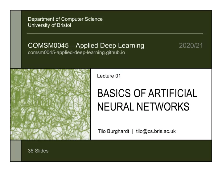
BASICS OF ARTIFICIAL NEURAL NETWORKS Tilo Burghardt | - PowerPoint PPT Presentation
Department of Computer Science University of Bristol COMSM0045 Applied Deep Learning 2020/21 comsm0045-applied-deep-learning.github.io Lecture 01 BASICS OF ARTIFICIAL NEURAL NETWORKS Tilo Burghardt | tilo@cs.bris.ac.uk
Department of Computer Science University of Bristol COMSM0045 – Applied Deep Learning 2020/21 comsm0045-applied-deep-learning.github.io Lecture 01 BASICS OF ARTIFICIAL NEURAL NETWORKS Tilo Burghardt | tilo@cs.bris.ac.uk 35 Slides
Agenda for Lecture 1 • Neurons and their Structure • Single & Multi Layer Perceptron • Basics of Cost Functions • Gradient Descent and Delta Rule • Notation and Structure of Deep Feed-Forward Networks Lecture 1 | 2 Applied Deep Learning | University of Bristol
Biological Inspiration Lecture 1 | 3 Applied Deep Learning | University of Bristol
Golgi’s first Drawings of Neurons CAMILLO GOLGI Computation in biological neural networks is delivered based on the co-operation of individual computational components , namely neuron cells. image source: www.the-scientist.com Lecture 1 | 4 Applied Deep Learning | University of Bristol
Schematic Model of a Neuron myelin sheath axon axon terminals cell body nucleus dendrites main flow of information: feed-forward synapse Lecture 1 | 5 Applied Deep Learning | University of Bristol
Pavlov and Assistant Conditioning a Dog An environment can condition the behaviour of biological neural networks leading to the incorporation of new information. image source: www.psysci.co Lecture 1 | 6 Applied Deep Learning | University of Bristol
Neuro-Plasticity • plasticity refers to a system’s ability to adapt structure and/or behaviour to accommodate new information • the brain shows various forms of plasticity: - natural forms include synaptic plasticity (mainly chemical) , structural sprouting (growth) , rerouting (functional changes) , and neurogenesis (new neurons) temporal system evolution image source: Example of structural sprouting. www.cognifit.com Lecture 1 | 7 Applied Deep Learning | University of Bristol
Artificial Feed-forward Networks Lecture 1 | 8 Applied Deep Learning | University of Bristol
Rosenblatt’s (left) development of the Perceptron (1950s) image source: csis.pace.edu Lecture 1 | 9 Applied Deep Learning | University of Bristol
Simplification of a Neuron to a Computational Unit input x multiplication flow of information: feed-forward with weights w x 1 summation w 1 activation function input width w 2 x 2 ∑ sign y output w 3 x 3 ... y sign w x b i i ... i 1 if v 0 - b sign ( v ) def 1 otherwise bias Lecture 1 | 10 Applied Deep Learning | University of Bristol
Notational Details for the Perceptron unit function y=f (x) is shorthand for f (x;w) w 0 -1 bias s y w 1 x 1 ∑ g output w 2 CONVENTION: bias is x 2 incorporated ... in parameter vector activation function g summation ... various w [ w w ...] θ [ ...] different input parameters 0 1 0 1 variable names are used for parameters, most often we T T y sign ( w x ) g ( w x ) will use w parameters input unit output activation function NOTATION: a minor letter in non-italic NOTATION: NOTATION: f ( x ; w ) font refers to a semicolon italic font vector, a capital separates input refers to letter in non-italic input (left) from parameters scalars unit function font would refer to a parameters matrix or vector set (right) Lecture 1 | 11 Applied Deep Learning | University of Bristol
Geometrical Interpretation of the State Space T 0 w x The basic Perceptron defines a hyper plane . in x -state space that linearly separates x 2 two regions of that space (which corresponds to a two-class normal linear classification) w 0 /w 2 vector w 2 w 1 positive sign area negative sign area T w x 0 T w x 0 x 1 w 0 /w 1 T w x 0 hyper plane hyper plane defined by parameters w acts as decision boundary Lecture 1 | 12 Applied Deep Learning | University of Bristol
Basic Perceptron (Supervised) Learning Rule • Idea: whenever the system produces a misclassification with current weights, w adjust weights by towards a better performing weight vector: ground truth actual output * if * f ( x ) x f ( x ) f ( x ) w otherwise 0 update ... where is the learning rate. Lecture 1 | 13 Applied Deep Learning | University of Bristol
Training a Single-Layer Perceptron Compare Output and Ground Truth * f ( x ) f ( x ) ? Compute Output Adjust Weights * if * f ( x ) x f ( x ) f ( x ) T f (x) sign ( w x ) i w i otherwise 0 Consider Next (Training) Input Pair * x , f ( x ) Lecture 1 | 14 Applied Deep Learning | University of Bristol
Perceptron Learning Example: OR Perceptron Training Attempt of OR using * w ( f ( x ) f ( x )) x ; 0 . 5 OR x 0 x 1 x 2 parameters w f f* update ∆ w x 1 x 2 f* learning progress sampling some ( x , f*) -1 0 0 (0,0,0) 1 -1 (1,0,0) 0 0 -1 -1 1 0 (1,0,0) -1 1 (-1,1,0) 0 1 1 -1 0 0 (0,1,0) 1 -1 (1,0,0) 1 0 1 -1 0 1 (1,1,0) -1 1 (-1,0,1) 1 1 1 -1 0 0 (0,1,1) 1 -1 (1,0,0) -1 0 1 (1,1,1) 1 1 (0,0,0) encoding could be -1 1 0 (1,1,1) 1 1 (0,0,0) changed to traditional value 0 by adjusting -1 1 1 (1,1,1) 1 1 (0,0,0) the output of the sign function to 0; training -1 0 0 (1,1,1) -1 -1 (0,0,0) algorithm still valid ... ... ... ... ... ... ... Lecture 1 | 15 Applied Deep Learning | University of Bristol
Geometrical Interpretation of OR Space Learned x 2 class label 1 1 1 1= w 0 /w 2 positive sign area T w x 0 x 1 -1 1 1= w 0 /w 1 negative sign area class label -1 T T w x 0 w x 0 hyper plane defined by weights Lecture 1 | 16 Applied Deep Learning | University of Bristol
Larger Example Visualisation image source: datasciencelab.wordpress.com Lecture 1 | 17 Applied Deep Learning | University of Bristol
Cost Functions Lecture 1 | 18 Applied Deep Learning | University of Bristol
Cost (or Loss) Functions Idea: Given a set X of input vectors x of one or more variables and a parameterisation w , a Cost Function is a map J onto a real number representing a cost or loss associated with the input configurations. (Negatively related to ‘goodness of fit’.) * Expected Loss: J ( X; w ) L ( f ( x; w ), f ( x )) * ( x, f ( x )) ~ p 1 * Empirical Risk: J ( X; w ) L ( f ( x; w ), f ( x )) | X | x X 1 2 * MSE Example: MSE J ( X; w ) f ( x; w ) f ( x ) loss | X | x X loss function per example loss function Lecture 1 | 19 Applied Deep Learning | University of Bristol
Energy Landscapes over Parameter Space Cost Function J parameter dimensions of w Lecture 1 | 20 Applied Deep Learning | University of Bristol
Steepest Gradient Descent Lecture 1 | 21 Applied Deep Learning | University of Bristol
Idea of ‘Steepest’ Gradient Descent w w J ( X; w ) t 1 t t learning rate new old steepest gradient parameter dimensions of w Lecture 1 | 22 Applied Deep Learning | University of Bristol
The Delta Rule 1 2 MSE-type cost function T * J ( X; w ) w x f ( x ) with identity function as 2 | X | activation function x X weight vector change is w J ( X; w ) modelled as a move along change for a the steepest descent single weight w k J ( X; w ) T * w x w x f ( x ) k k w | X | x X k ...and for a single sample... T * w x w x f ( x ) k k this term looks similar to the Perceptron learning rule T * w x w x f ( x ) is the error derivative w x also known as The Delta Rule (Widrow & Hoff, 1960) Lecture 1 | 23 Applied Deep Learning | University of Bristol
Linear Separability Lecture 1 | 24 Applied Deep Learning | University of Bristol
Basic Learning Example: XOR Perceptron Training Attempt of XOR using * w ( f ( x ) f ( x )) x ; 0 . 5 XOR x 0 x 1 x 2 parameters f f* update x 1 x 2 f* learning progress sampling some ( x , f*) -1 0 0 (0,0,0) 1 -1 (1,0,0) 0 0 -1 -1 1 0 (1,0,0) -1 1 (-1,1,0) 0 1 1 -1 0 0 (0,1,0) 1 -1 (1,0,0) 1 0 1 -1 0 1 (1,1,0) -1 1 (-1,0,1) 1 1 -1 -1 0 0 (0,1,1) 1 -1 (1,0,0) -1 0 1 (1,1,1) 1 1 (0,0,0) Will the -1 1 0 (1,1,1) 1 1 (0,0,0) learning -1 1 1 (1,1,1) 1 -1 (1,-1,-1) process -1 1 0 (1,0,0) -1 1 (-1,1,0) ever produce a -1 0 1 (1,1,0) -1 1 (-1,0,1) solution? ... ... ... ... ... ... ... Lecture 1 | 25 Applied Deep Learning | University of Bristol
Recommend
More recommend
Explore More Topics
Stay informed with curated content and fresh updates.
