Basic Probability and Statistics CS540 Bryan R Gibson University of - PowerPoint PPT Presentation

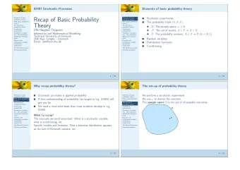
Basic Probability and Statistics CS540 Bryan R Gibson University of Wisconsin-Madison Slides adapted from those used by Prof. Jerry Zhu, CS540-1 1 / 35

Reasoning with Uncertainty ◮ There are two identical-looking envelopes ◮ one has a red coin (worth $100) and a black coin (worth $0) ◮ the other has two black coins ◮ You randomly grab an envelope and randomly pick out one coin - it’s black ◮ You’re then given the chance to switch envelopes: Should you? 2 / 35

Outline Probability: ◮ Sample Space ◮ Random Variables ◮ Axioms of Probability ◮ Conditional Probability ◮ Probabilistic Inference: Bayes Rule ◮ Independence ◮ Conditional Independence 3 / 35

Uncertainty ◮ Randomness ◮ Is our world random? ◮ Uncertainty ◮ Ignorance (practical and theoretical) ◮ Will my coin flip end in heads? ◮ Will a pandemic flu strike tomorrow? ◮ Probability is the language of uncertainty ◮ A central pillar of modern day A.I. 4 / 35

Sample Space ◮ A space of Events that we assign probabilities to ◮ Events can be binary, multi-valued or continuous ◮ Events are mutually exclusive ◮ Examples: ◮ Coin flip: { head,tail } ◮ Die roll: { 1,2,3,4,5,6 } ◮ English words: a dictionary ◮ Temperature tomorrow: R + (kelvin) 5 / 35

Random Variable ◮ A variable X , whose domain is the sample space, and whose value is somewhat uncertain ◮ Examples: ◮ X = coin flip outcome ◮ X = first word in tomorrow’s headline news ◮ X = tomorrow’s temperature ◮ Kind of like x = rand() 6 / 35

Probability for Discrete Events ◮ Probability P ( X = a ) is the fraction of times X takes value a ◮ Often written as P ( a ) ◮ There are other definitions of prob. and philosophical debates, but we’ll set those aside for now ◮ Examples: ◮ P ( head ) = P ( tail ) = 0 . 5 : a fair coin ◮ P ( head ) = 0 . 51 , P ( tail ) = 0 . 49 : a slightly biased coin ◮ P ( head ) = 1 , P ( tail ) = 0 : Jerry’s coin ◮ P ( first word = “the” when flip to random page in R&N ) =? ◮ Demo: bookofodds 7 / 35

Prob. for Discrete Events (cont.) : Probability Table ◮ Example: Weather sunny cloudy rainy 200/365 100/365 65/365 ◮ P ( Weather = sunny ) = P ( sunny ) = 200 365 � 200 365 , 100 365 , 65 ◮ P ( Weather ) = � 365 ◮ (For now, we’ll be satisfied with just using counted frequency of data to obtain probabilities . . . ) 8 / 35

Prob. for Discrete Events (cont.) ◮ Probability for more complex events : we’ll call it event A ◮ P ( A = “head or tail” ) =? (for a fair coin?) ◮ P ( A = “even number” ) =? (for a fair 6-sided die?) ◮ P ( A = “two dice rolls sum to 2” ) =? 9 / 35

Prob. for Discrete Events (cont.) ◮ Probability for more complex events : we’ll call it event A ◮ P ( A = “head or tail” ) = 1 2 + 1 2 = 1 (fair coin) ◮ P ( A = “even number” ) = 1 6 + 1 6 + 1 6 = 1 2 (fair 6-sided die) ◮ P ( A = “two dice rolls sum to 2” ) = 1 6 · 1 1 6 = 36 10 / 35

The Axioms of Probability ◮ P ( A ) ∈ [0 , 1] ◮ P ( true ) = 1 , P ( false ) = 0 ◮ P ( A ∨ B ) = P ( A ) + P ( B ) − P ( A ∧ B ) 11 / 35

The Axioms of Probability (cont.) ◮ P ( A ) ∈ [0 , 1] Sample Space No fraction of A can be smaller than 0 12 / 35

The Axioms of Probability (cont.) ◮ P ( A ) ∈ [0 , 1] Sample Space No fraction of A can be bigger than 1 13 / 35

The Axioms of Probability (cont.) ◮ P ( true ) = 1 , P ( false ) = 0 Sample Space Valid sentence: e.g. “ x = head OR x = tail” 14 / 35

The Axioms of Probability (cont.) ◮ P ( true ) = 1 , P ( false ) = 0 Sample Space Invalid sentence: e.g. “ x = head AND x = tail” 15 / 35

The Axioms of Probability (cont.) ◮ P ( A ∨ B ) = P ( A ) + P ( B ) − P ( A ∧ B ) Sample Space A B 16 / 35

Some Theorems Derived from Axioms ◮ P ( ¬ A ) = 1 − P ( A ) A ◮ If A can take k different values a 1 , . . . , a k : P ( A = a 1 ) + . . . + P ( A = a k ) = 1 ◮ If A is a binary event: P ( B ) = P ( B ∧ ¬ A ) + P ( B ∧ A ) ◮ If A can take k values: � P ( B ) = P ( B ∧ A = a i ) i =1 ..k 17 / 35

Joint Probability ◮ Joint Probability: P ( A = a, B = b ) , shorthand for P ( A = a ∧ B = b ) , is the probability of both A = a and B = b happening P ( A = a ) : e.g. P ( 1st word = “San” ) = 0.001 P ( B = b ) : e.g. P ( 2nd word = “Francisco” ) = 0.0008 A B P ( A = a, B = b ) : e.g. P ( 1st = “San”, 2nd = “Francisco” ) = 0.0007 18 / 35

Joint Probability Table Weather sunny cloudy rainy hot 150/365 40/365 5/365 Temp cold 50/365 60/365 60/365 ◮ P ( Temp = hot, Weather = rainy ) = P ( hot, rainy ) = 5 / 365 ◮ The full joint probability table between N variables, each taking k values, has k N entries! 19 / 35

Marginal Probability ◮ Marginalize = Sum over “other” variables ◮ For example, marginalize over/out Temp: Weather sunny cloudy rainy hot 150/365 40/365 5/365 Temp cold 50/365 60/365 60/365 � 200/365 100/365 65/365 � 200 365 , 100 365 , 65 � P ( Weather ) = 365 ◮ “Marginalize” comes from old practice of writing sums in margin 20 / 35

Marginal Probability (cont.) ◮ Marginalize = Sum over “other” variables ◮ Now marginalize over Weather: Weather sunny cloudy rainy � hot 150/365 40/365 5/365 195/365 Temp cold 50/365 60/365 60/365 170/365 � 195 365 , 170 � P ( Temp ) = 365 ◮ This is nothing but P ( B ) = � i =1 ..k P ( B ∧ A = a i ) if A can take k values 21 / 35

Conditional Probability ◮ P ( A = a | B = b ) : fraction of times A=a within the region that B=b, or given that B=b P ( A = a ) : e.g. P ( 1st word = “San” ) = 0.001 P ( B = b ) : e.g. P ( 2nd word = “Francisco” ) = 0.0008 A B P ( A = a | B = b ) : e.g. P ( 1st = “San” | 2nd = “Francisco” ) = 0.875 Although both “San” and “Fransisco” are rare, given “Francisco”, “San” quite likely! 22 / 35

Conditional Probability (cont.) ◮ In general, conditional probability is defined P ( A = a | B ) = P ( A = a, B ) P ( A = a, B ) = P ( B ) � all a i P ( A = a i , B ) ◮ We can have everything conditioned on some other events C, to get a conditional version of conditional probability: P ( A | B, C ) = P ( A, B | C ) P ( B | C ) This should be read as P ( A | ( B, C )) 23 / 35

The Chain Rule ◮ From the definition of conditional probability we get the chain rule: P ( A, B ) = P ( A | B ) P ( B ) = P ( B | A ) P ( A ) ◮ It works for more than two items too: P ( A 1 , A 2 , . . . , A n ) = P ( A 1 ) P ( A 2 | A 1 ) P ( A 3 | A 1 , A 2 ) . . . P ( A n | A 1 , A 2 , . . . , A n − 1 ) 24 / 35

Reasoning ◮ How do we use probabilities in A.I.? ◮ Example: ◮ You wake up with a headache ◮ Do you have the flue? ◮ H = headache, F = flu ◮ Logical Inference: if H then F . (world often not this clear) ◮ Statistical Inference: compute probability of a query given (or conditioned on) evidence, i.e. P ( F | H ) 25 / 35

Inference with Bayes’ Rule: Example 1 ◮ Inference: compute the probability of a query given evidence ◮ H = have headache, F = have flu ◮ You know that: P ( H ) = 0 . 1 “1 in 10 people has a headache” P ( F ) = 0 . 01 “1 in 100 people has the flu” P ( H | F ) = 0 . 9 “90% of people who have flu have headache” ◮ How likely is it that you have the flu? ◮ 0.9? ◮ 0.01? ◮ . . . ? 26 / 35

Inference with Bayes’ Rule: Example 1 (cont.) Bayes Rule in Essay Towards Solving a Problem in the Doctrine of Chances (1764) P ( F | H ) = P ( F, H ) = P ( H | F ) P ( F ) P ( H ) P ( H ) Using: P ( H ) = 0 . 1 “1 in 10 people has a headache” P ( F ) = 0 . 01 “1 in 100 people has the flu” P ( H | F ) = 0 . 9 “90% of people who have flu have headache” We find: P ( F | H ) = 0 . 9 ∗ 0 . 01 = 0 . 09 0 . 1 ◮ So there’s a 9% chance you have the flu – much less than 90% ◮ But it’s higher than P ( F ) = 1% , since you have a headache 27 / 35

Inference with Bayes’ Rule (cont.) ◮ Bayes Rule P ( A | B ) = P ( A, B ) = P ( B | A ) P ( A ) P ( B ) P ( B ) ◮ Why make things so complicated? ◮ Often P ( B | A ) , P ( A ) and P ( B ) are easier to get ◮ Some terms: ◮ prior P ( A ) : probability before any evidence ◮ likelihood P ( B | A ) : assuming A, how likely is evidence ◮ posterior P ( A | B ) : conditional prob. after knowing evidence ◮ inference: deriving unknown probs. from known ones ◮ In general, if we have full joint prob. table, we can simply do: P ( A | B ) = P ( A, B ) more on this later . . . P ( B ) 28 / 35

Inference with Bayes’ Rule: Example 2 ◮ There are two identical-looking envelopes ◮ one has a red coin (worth $100) and a black coin (worth $0) ◮ the other has two black coins ◮ You randomly grab an envelope and randomly pick out one coin - it’s black ◮ You’re then given the chance to switch envelopes: Should you? 29 / 35

Inference with Bayes’ Rule: Example 2 (cont.) ◮ E : envelope, 1=(R,B), 2=(B,B) ◮ B : event of drawing a black coin P ( E | B ) = P ( B | E ) P ( E ) P ( B ) ◮ We want to compare P ( E = 1 | B ) vs. P ( E = 2 | B ) ◮ P ( B | E = 1) = 0 . 5 , P ( B | E = 2) = 1 ◮ P ( E = 1) = P ( E = 2) = 0 . 5 ◮ P ( B ) = 3 4 (and in fact we don’t need this for the comparison) ◮ P ( E = 1 | B ) = 1 3 , P ( E = 2 | B ) = 2 3 ◮ After seeing a black coin, the posterior probability of the this envelope being 1 (worth $100) is smaller than it being 2 ◮ You should switch! 30 / 35