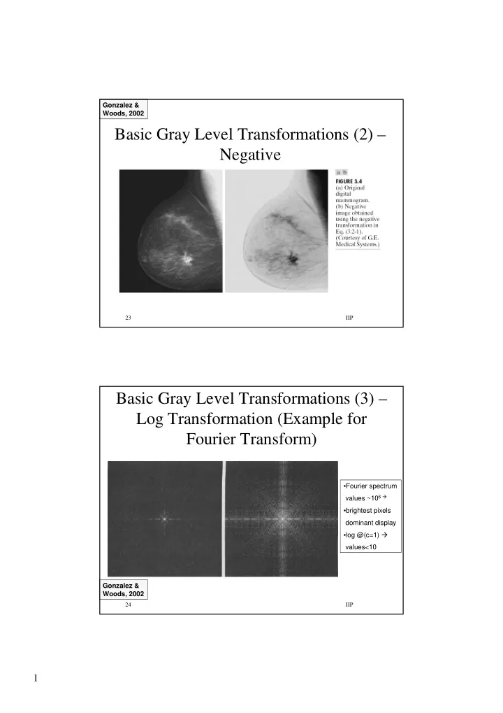
Basic Gray Level Transformations (2) Negative 23 IIP Basic Gray - PDF document

Gonzalez & Woods, 2002 Basic Gray Level Transformations (2) – Negative 23 IIP Basic Gray Level Transformations (3) – Log Transformation (Example for Fourier Transform) • Fourier spectrum values ~10 6 � • brightest pixels dominant display • log @(c=1) � values<10 Gonzalez & Woods, 2002 24 IIP 1

Basic Gray Level Transformations (4) – Power-Law Transformation (1) Gonzalez & Woods, 2002 25 IIP Basic Gray Level Transformations (5) – Power-Law Transformation (2) Gonzalez & Woods, 2002 26 IIP 2

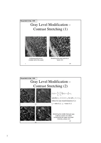
Basic Gray Level Transformations (6) – Gonzalez & Contrast Stretching Woods, 2002 poor illumination, lack of dynamic range in sensor … � low contrast image solution : increase dynamic range by piecewise linear transformation that cab be arbitrarily complex, however relies on the user = = r s , r s 1 1 2 2 ⇒ linear = = = − r r , s 0, s L 1 1 2 1 2 ⇒ thresholding threshold @ mean (d) = = −  ⇒ (c) ( , r s ) ( r ,0) and ( , r s ) ( r , L 1) [ ] − 1 1 min 2 2 max  linear stretch to 0, L 1  r & r the minimum & maximum GL min max 27 IIP Image Enhancement in the Spatial Domain – Histogram Equalization (HE) (1) • HE yields output image with equally many pixels at every gray level (flat histogram) which is useful before comparison/segmentation [ ] r ∈ • r – gray level in input image ( ) r normalized s.t 0,1 s = T ( r ) • s – gray level transformed by ( r,s =0 is black & r,s =1 is white) 28 IIP 3

HE (2) • Assume T ( r ) satisfies: a. T ( r ) is single-valued & monotonically ≤ r ≤ increasing in 0 1 ≤ ≤ ≤ ≤ 0 T r ( ) 1 for 0 r 1 (monotonicity) b. ⇒ • The inverse transform = − ≤ ≤ 1 ( ), 0 r T s s 1 exists (a) and the increasing order from black to white (a) and range (b) are preserved 29 IIP HE (3) • Viewed as random variables in [0,1], the gray levels are characterized by the (different) probability density functions (PDFs) p ( r ) and p ( s ) r s “dark” “light” image image 30 IIP 4

HE (4) • Following probability theory, if p ( r ) and p ( s ) r s 1 s T − are known and satisfies condition (a) ( ) then the PDF of the transformed gray levels is given by dr = (1) p p ( ) s ( ) r ds s r • The following enhancement techniques are based on modifying the appearance of an image by controlling the PDF of its gray levels via the transformation function T ( r ). 31 IIP HE (5) • Consider the (important in IP) transformation r ∫ = = ≤ ≤ p ( 2 ) s T ( r ) ( w ) dw , 0 r 1 r 0 which is the cumulative distribution function (CDF) of r . Since (1) the pdf is always positive, integral=area and T is single valued � condition (a); (2) integral of a pdf in [0,1] is also in [0,1] � (b), that is, the two conditions above are satisfied (check for yourself) 32 IIP 5

HE (6) • Solving (1) for the transformation in (2) yields dr 1 = = p p p ( ) s ( ) r ( ) r ds s r ds r dr 1 1 = = p p ( ) r ( ) r   dT r ( ) r r r d ∫  p  ( ) w dw dr dr   r 0 1 = = ≤ ≤ p ( ) r 1 0 s 1 r ( ) p r r • That is, the CDF transformation yields a random variable, s , having a uniform probability density (thus increasing the gray level dynamic range). Notice, is always p s s ( ) uniform independent of the form of . p r r ( ) 33 IIP HE (7) – Example (Continuous Case) − + ≤ ≤  2 r 2 0 r 1 =  p r ( r )  0 otherwise ∫ r = = − + s T ( r ) ( 2 w 2 ) dw 0 = − + 2 r 2 r dr dr = = − + = p p ( ) s ( ) r ( 2 r 2) s r ds ds = − = ± − 1 ( )   r T s 1 1 s d   − − − + − − =   2(1 1 s ) 2 (1 1 s )     = − − ds 1 1 s   d   − − − = ≤ ≤   2( 1 s ) (1 1 s ) 1 0 s 1   r ∈   ds [0,1] 34 IIP 6

HE (8) → ∑ ∫ • For digital images – density � probability, • The probability of occurrence of gray level is r k n = p ≤ ≤ = − ( ) r k , 0 r 1, k 0, L 1 for levels L n k k r n is the total number of pixels in the image and n is the number of pixels having gray level r k k • The discrete version of the CDF transformation k k ∑ ∑ n = = = = − j s T r ( ) p r ( ) , k 0, L 1 k k r j n = = j 0 j 0 This transformation is called histogram equalization (show that T satisfies both conditions) 35 IIP HE (9) • Unlike for the continuous transformation, it cannot be proved that this discrete transformation will produce the discrete equivalent of a uniform pdf, which would be a uniform histogram. However, it does have the tendency of spreading the histogram so that the levels of the histogram-equalized image will span a fuller range of the gray scale 36 IIP 7

HE (10) Advantages: • Gray level span the entire range • Automatic (based on image; no parameter selection) • Simple to calculate 37 IIP Gonzalez & Wintz, 1977 HE (11) – Example (Discrete Case) (1) • 64x64, 8-level image having the following distribution 0 ∑ = = = = s T ( r ) p ( r ) p ( r ) 0 . 19 0 0 r j r 0 = j 0 1 ∑ = = = s T r ( ) p r ( ) 1 1 r j = j 0 + = p r ( ) p r ( ) 0.44 0 1 r r = = = s 0.65, s 0.81, s 0.89, 2 3 4 = = = s 0.95, s 0.98, s 1.00 5 6 7 (Fig. a) 38 IIP 8

HE (12) – Example (Discrete Case) (2) • Only eight equally-spaced levels are allowed, thus each of the transformed values must be assigned to its closest valid level ≅ ≅ ≅ ≅ s 1/ 7, s 3/ 7, s 5/ 7, s 6/ 7, 0 1 2 3 ≅ ≅ ≅ ≅ s 6/ 7, s 1, s 1, s 1 (Fig. b) 4 5 6 7 • There are only 5 distinct histogram-equalized gray levels, thus redefinition yields the levels = = = = = s 1 / 7 , s 3 / 7 , s 5 / 7 , s 6 / 7 , s 1 0 1 2 3 4 = = 790 pixels @ s 1/ 7, 1023 pixels @ s 3/ 7, 0 1 = + = = 850 pixels @ s 5/ 7, 656 329 985 pixels @ s 6/ 7, 2 3 + + = = 245 122 81 448 pixels @ s 1 (Fig. c) 4 39 IIP HE (13) – Example (Discrete Case) (3) 40 IIP 9

Castleman, 1996 HE (10) – Illustration 1 output image with equally many pixels at every gray level 41 IIP Gonzalez & Wintz, 1977 HE (11) – Illustration 2 42 IIP 10

Gonzalez & Woods, 2002 1 HE (12) – Illustration 3 2 3 4 43 IIP 11