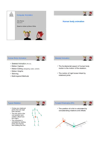
Basic Animation Techniques Graphics & Visualization: Principles - PowerPoint PPT Presentation

Graphics & Visualization Chapter 17 Basic Animation Techniques Graphics & Visualization: Principles & Algorithms Chapter 17

Introduction • Animate : to give life. • Computer animation: “life” given by presenting a sequence of still images ( frames ) in rapid succession: � If frames presented at sufficiently high rate � human eye-brain perceives them as smooth motion or animation • Minimum rate required for smooth motion ≈ 12 fps : � Below that, motion appears jerky • Generally required fps is not constant; it depends on speed of movement of the objects as well as on illumination parameters • History 19 th century: � Celluloid film (Goodwin 1887) � Kinetoscope (Edison, 1893) � Cinematograph (Lumiere, 1894) 2 Graphics & Visualization: Principles & Algorithms Chapter 17

Introduction (2) • History 20 th century: � Enchanted Drawing & Humorous Phases of Funny Faces (Blackton, 1900) � Fantasmagorie (Cohl, 1908) � Little Nemo (McCay, 1911) � Most cartoon animation was performed by tweening , the drawing of frames in-between key-frames ; replaced by computers using interpolation techniques � Tron and Star Trek (1982) � Tin Toy (1989) • Animation finds important applications in visualization • Computer animation created by altering a multitude of parameters that affect change between frames • Typical example: Observer parameters, position of objects within the scene, characteristics of the objects (color & size) 3 Graphics & Visualization: Principles & Algorithms Chapter 17

Introduction (3) • Parameters encoded in a large # of animation variables • Impossible for an animator to define every animation variable for every frame; animation control methods have been developed • Examples: Procedural & representational methods for animating rigid bodies & skeletal animation for animating human-like or animal-like characters • These methods use common low level techniques such as: � Interpolation, � Collision detection & � Motion blur • Higher level animation control methods examined: � Rigid body animation � Skeletal animation � Deformable models � Particle systems 4 Graphics & Visualization: Principles & Algorithms Chapter 17

Introduction (4) • Procedural animation: Refer to the encapsulation of the animation of an object in a procedure: � Animation sequences can automatically be generated, often in real-time � Particle systems : Largest subclass of procedural animation � Rigid body and Skeletal animation : Can also be done procedurally � Behavioral animation : Subclass of procedural animation where objects determine their own actions, taking into account their environment • Animation Examples: (a) Sequence of frames of a face changing expressions (b) Frames of a moving observer sequence 5 Graphics & Visualization: Principles & Algorithms Chapter 17

Low Level Animation Techniques • A lower layer of tools: � Interpolation techniques : � Means by which computer takes over the task of tweening � Collision detection: � Essential for realism by detecting when moving objects collide so that appropriate action can be taken � Anti-aliasing in time ( Motion blur ): essential to most animations � Morphing : � Allows smooth transition from one graphical object to another (in a # of frames) & is the successor to the well known effect of cross- fading in traditional motion pictures 6 Graphics & Visualization: Principles & Algorithms Chapter 17

Interpolation, Keyframes & Tweening • Before: � Experienced animators create key frames : � Significant changes in the animation variables (direction of motion) � Less experienced animators do the tweening work: � Fill the in-between frames to reach the desired frame rate (fps) � Tweening is less costly than keyframing • Today: � Animation uses interpolation to do the tweening work automatically � Extreme values of the animation variables are specified by the user � Values of animation variables are linked to frames of the animation: � Since there is a 1-1 mapping between frames & time, animation variables are linked to time � Use parametric functions f ( t ) to interpolate the animation variables between extreme values, e.g. v 0 & v 1 , which become the interpolation control points 7 Graphics & Visualization: Principles & Algorithms Chapter 17

Interpolation, Keyframes & Tweening (2) • Tweening between key-frames at t 0 & t 1 : • Care must be taken in selecting the variables to be interpolated : � Importance of animation variable selection, e.g.: Choosing (a) the endpoint and (b) the rotation angle as animation variable 8 Graphics & Visualization: Principles & Algorithms Chapter 17

Interpolation, Keyframes & Tweening (3) • Interpolation is based on a parameter t representing time • Interpolation functions pass through the interpolation control points, so f ( t 0 ) = v 0 , f ( t 1 ) = v 1 for some t 0 , t 1 • Simplest form of parametric interpolation: Linear interpolation : (17.1) = − + ∈ L t ( ) (1 t v ) tv t [0 ] ,1 0 1 • Linear interpolation is used frequently: � When more advanced change is required we employ more complex forms � Example: Smooth path of an object NOT moving in a straight line could be described better by a function such as Bezier • Quadratic Bezier function interpolates between control values v 0 and v 2 using an extra value v 1 as an attractor: (17.2) = − + − + ∈ 2 2 2 B t ( ) (1 t ) v 2 (1 t t v ) t v t [0, ] 1 0 1 2 9 Graphics & Visualization: Principles & Algorithms Chapter 17

Interpolation, Keyframes & Tweening (4) • The n th degree Bezier function interpolates between v 0 & v n using n -1 attractor values v i , i :1.. n-1 � These values attract the interpolation toward them & exert their max attraction at the i/n values of t • Functions of parametric curves X ( t ) are good interpolation functions: � Their tangent vector X '( t ) defines velocity � useful when used to describe motion � The arc length travelled along such a curve function can be computed by integrating velocity • Arc length travelled is not proportional to the time parameter t : � Can not use constant differences of t to get constant arc lengths of travel � Reparameterization of a curve function by arc length s is required 10 Graphics & Visualization: Principles & Algorithms Chapter 17

Interpolation, Keyframes & Tweening (5) • Points on curve for constant differences of the parameter t and, after reparameterization, for constant differences of parameter s: • Reparameterization by arc length NOT possible for every curve function: � Pre-computed set of arc lengths s i for points on the curve function can be used 11 Graphics & Visualization: Principles & Algorithms Chapter 17

Interpolation, Keyframes & Tweening (6) • Arc lengths between points on a curve: • Then point p ’ on the curve function that corresponds to arc length s ’ can be approximated by linearly interpolating the points of the 2 nearest arc lengths s i & s i+1 ( s i ≤ s’ ≤ s i+1 ): ′ ′ − − s s s s (17.3) ′ = + + i 1 i p p p + i i 1 − − s s s s + + i 1 i i 1 i 12 Graphics & Visualization: Principles & Algorithms Chapter 17

Interpolation of Rotation • Suppose we express an arbitrary rotation as a synthesis of 3 basic θ → θ → θ rotations ( ) ( ) ( ) R R R x x y y z z • Animate this by gradually incrementing θ x , θ y , θ z � problems: 1. Rather difficult to estimate basic rotation angles that make up the required rotation about an arbitrary axis 2. Encounter a “twisting” motion, as the rotations are applied sequentially & the object seems to rotate alternately about the 3 axes 3. Encounter a phenomenon known as gimbal lock 13 Graphics & Visualization: Principles & Algorithms Chapter 17

Interpolation of Rotation (2) • Solution: Use a composite rotation matrix about an arbitrary axis • Better Solution: Use quaternions • Quaternion rotation is more stable, requires fewer calculations & consecutive rotations can be handled in a smooth way • Two extreme positions of the rotation can be represented by 2 unit quaternions: � corresponding to the initial position and q = (1, ) 0 � 0 θ θ corresponding to the position after rotation by θ around = ˆ q (sin ,cos ) n � 1 2 2 the given axis with direction ˆ n • Linear interpolation between these 2 quaternions will not produce expected smooth rotation between the 2 positions: � Instead a motion that would accelerate towards the middle • Geometrically, unit quaternions representing rotations lie on the surface of the 4-D unit hypersphere � linear interpolation interpolates on the chord through them (see � ) 14 Graphics & Visualization: Principles & Algorithms Chapter 17