Background Poisson or Binomial data with the following properties - PowerPoint PPT Presentation

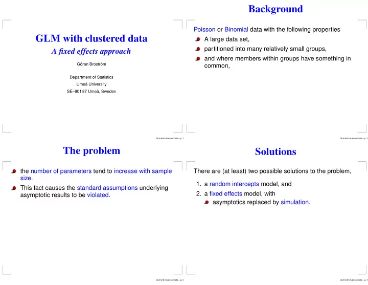
Background Poisson or Binomial data with the following properties GLM with clustered data A large data set, partitioned into many relatively small groups, A fixed effects approach and where members within groups have something in G¨ oran Brostr¨ om common, Department of Statistics Ume˚ a University SE–901 87 Ume˚ a, Sweden GLM with clustered data – p. 1 GLM with clustered data – p. 2 The problem Solutions the number of parameters tend to increase with sample There are (at least) two possible solutions to the problem, size. 1. a random intercepts model, and This fact causes the standard assumptions underlying 2. a fixed effects model, with asymptotic results to be violated. asymptotics replaced by simulation. GLM with clustered data – p. 3 GLM with clustered data – p. 4

Packages in R Data structure The package Matrix has lmer, n clusters of sizes n i , i = 1 , . . . , n . the MASS package has glmmPQL, For each cluster i, i = 1 , . . . , n , observe responses ( y i 1 , . . . , y in i ) and Jim Lindsey’s glmm in his repeated package, vectors of explanatory variables ( x i 1 , . . . , x in i ) , where x ij Myles’ and Clayton’s GLMMGibbs for fitting mixed are p -dimensional vectors with models by Gibbs sampling. the first element identically equal to unity, Adding to that glmmML and glmmboot in the package corresponding to the mean value of the random glmmML. intercepts. The random part, u i of the intercepts are normal with mean zero and variance σ 2 , and it is assumed that u 1 , . . . , u n are independent. GLM with clustered data – p. 5 GLM with clustered data – p. 6 The conditional distribution Likelihood function given the random intercepts β 1 + u i , i = 1 , . . . , n : In the fixed effects model (and in the conditional random effects model), the likelihood function is Pr ( Y ij = y ij | u i ; x ) = P ( β x ij + u i , y ij ) , n n i y ij = 0 , 1 , . . . ; j = 1 , . . . , n i , i = 1 , . . . , n. � � � � L ( β , γ ); y , x = P ( β x ij + γ i , y ij ) . i =1 j =1 Bernoulli distribution logit link, The log likelihood function is e xy P ( x, y ) = 1 + e x , y = 0 , 1; −∞ < x < ∞ , n n i cloglog link � � � � ℓ ( β , γ ); y , x = log P ( β x ij + γ i , y ij ) , ´ y exp 1 − exp( − e x ) − (1 − y ) e x ´ i =1 j =1 ` ` P ( x, y ) = , y = 0 , 1; −∞ < x < ∞ , Poisson distribution with log link P ( x, y ) = e xy y ! e − e x , y = 0 , 1 , 2 , . . . ; −∞ < x < ∞ GLM with clustered data – p. 7 GLM with clustered data – p. 8

Computational aspects Tests of cluster effect Testing is performed via a simple bootstrap (glmmboot). A profiling approach reduces an optimizing problem in Under the null hypothesis of no grouping effect, high dimensions the grouping factor can be randomly permuted without to a problem consisting of changing the probability distribution (the conditional solving several one-variable equations followed by approach), or optimization in low dimensions. a parametric bootstrap approach: simulate observations from the fitted model under the null hypothesis (the unconditional approach). GLM with clustered data – p. 9 GLM with clustered data – p. 10 Cluster components of the score The score vector The partial derivatives wrt β m , m = 1; . . . , p , of the log The partial derivatives wrt γ i , i = 1 , . . . , n , are likelihood function are: U p + i ( β , γ ) = ∂ � � ℓ ( β , γ ); y , x ∂ ∂γ i � � U m ( β , γ ) = ℓ ( β , γ ); y , x ∂β m n i � n n i = G ( β x ij + γ i , y ij ) , i = 1 , . . . , n. � � = x ijm G ( β x ij + γ i , y ij ) , m = 1 , . . . , p. j =1 i =1 j =1 where ∂ ∂x P ( x, y ) G ( x, y ) = ∂ ∂x log P ( x, y ) = P ( x, y ) GLM with clustered data – p. 11 GLM with clustered data – p. 12

With profiling Profile score Setting U p + i ( β , γ ) = 0 defines γ implicitly as functions of β , ∂F γ i = γ i ( β ) , i = 1 , . . . , n : ∂γ i ( β ) ∂β m = − ∂F ∂β m n i ∂γ i � � � � � F β , γ i ( β ) = G β x ij + γ i ( β ) , y ij = 0 , i = 1 , . . . , n. � n i � � j = i x ijm H β x ij + γ i , y ij = − , i = 1 , . . . , n ; m = 1 , . . . , j =1 � n i � � j =1 H β x ij + γ i , y ij From ∂ = ∂γ i ∂F + ∂F which is needed when calculating the score corresponding � � F β , γ i ( β ) = 0 to the profile likelihood. ∂β m ∂β m ∂γ i ∂β m we get GLM with clustered data – p. 13 GLM with clustered data – p. 14 Profile loglihood Profile partial derivatives The partial derivatives wrt β m , m = 1; . . . , p , of the log Replacing γ by γ ( β ) gives the profile log likelihood ℓ ( P ) : profile likelihood function becomes: n n i ℓ ( P ) � � � � � � β ; y , x = log P β x ij + γ i ( β ) , y ij , ∂ U ( P ) ℓ ( P ) ( β ; y , x ) m ( β ) = i =1 j =1 ∂β m n n i � x ijm + ∂γ i ( β ) � as a function of β alone. � � � � = G β x ij + γ i ( β ) , y ij ∂β m i =1 j =1 n n i ∂γ i ( β ) � � � � � � = U m β , γ ( β ) + G β x ij + γ i ( β ) , y ij ∂β m i =1 j =1 = U m ( β , γ ( β )) , Thus we get back the unprofiled partial derivatives. GLM with clustered data – p. 15 GLM with clustered data – p. 16

Profile hessian At the maximum Justifying the use of the profile likelihood: ∂ − I ( P ) Theorem 1 (Patefield) The inverse hessians from the full � � ms ( β ) = β , γ ( β ) U m ∂β s likelihood and from the profile likelihood for β are equal n n i � x ijs + ∂γ i ( β ) � when � � � � = x ijm H β x ij + γ i ( β ) , y ij ∂β s γ , ˆ ( γ , β ) = (ˆ β ) . i =1 j =1 = − I ms ( β , γ ( β )) � n i � n i n j =1 x ijm H ij j =1 x ijs H ij � − , � n i j =1 H ij i =1 m, s = 1 , . . . , p. where � � H ij = H β x ij + γ i ( β ) , y ij , j = 1 , . . . n i ; i = 1 , . . . , n. GLM with clustered data – p. 17 GLM with clustered data – p. 18 Preparation for R Implementation in R ℓ ( P ) ( β ) = � n � n i Implemented in the package glmmML in R . � � j =1 log P β x ij + γ i ( β ) , y ij , i =1 Covers three cases, U ( P ) m ( β ) = � n � n i � � , j =1 x ijm G β x ij + γ i ( β ) , y ij i =1 1. Binomial with logit link, m = 1 , . . . , p. 2. Binomial with cloglog link, For fixed β , γ i ( β ) is found by solving 3. Poisson with log link. n i The function is glmmboot, � G ( β x ij + γ i , y ij ) = 0 , Testing of cluster effect is done by simulation (a simple j =1 form of bootstrapping). with respect to γ i , i = 1 , . . . , n . conditionally, or unconditionally. The maximization is performed by optim, via the C function vmmin, available as an entry point in the C code of R . GLM with clustered data – p. 19 GLM with clustered data – p. 20

Binomial with logit link Binomial with cloglog link P ( x, y ) = (1 − exp( − exp( x )) y exp( − (1 − y ) exp( x )) , P ( x, y ) = exp( xy ) / (1 + exp( x )) , G ( x, y ) = y − P ( x, 1) . G ( x, y ) = exp( x ) P ( x, 1) { y − P ( x, 1) } We get ( γ 1 , . . . , γ n ) by solving the equations We get ( γ 1 , . . . , γ n ) by solving the equations n i n i exp( β x ij + γ i ) n i n i � � y ij = � � y ij = n i − exp( − exp( β x ij + γ i )) 1 + exp( β x ij + γ i ) j =1 j =1 j =1 j =1 for i = 1 , . . . , n (using the C version of uniroot ). for i = 1 , . . . , n (using the C version of uniroot ). Special cases: � y ij = 0 or n i ; giving γ i = −∞ or + ∞ , Special cases: � y ij = 0 or n i ; γ i = −∞ or + ∞ , respectively. respectively. Corresponding cluster can be thrown out. Corresponding cluster can be thrown out. (Should be used in glm ?) GLM with clustered data – p. 21 GLM with clustered data – p. 22 Poisson with log link Simulation P ( x, y ) = e xy Model: y ! exp( − exp( x )) G ( x, y ) = y − e x P ( Y ij = 1 | γ i ) = 1 − P ( Y ij = 0 | γ i ) e γ i We get ( γ 1 , . . . , γ n ) from = 1 + e γ i , j = 1 , . . . , 5; i = 1 , . . . , n, n i n i � y ij = e γ i � where γ 1 , . . . , γ n are iid N (0 , σ ) . exp( β x ij ) , i = 1 , . . . , n, j =1 j =1 Hypothesis: σ = 0 . giving � j y ij � � γ i = log , i = 1 , . . . , n. � j exp( β x ij ) Special case: � y ij = 0 , giving γ i = −∞ . GLM with clustered data – p. 23 GLM with clustered data – p. 24