Background Background Require computationally efficient scheme to - PDF document

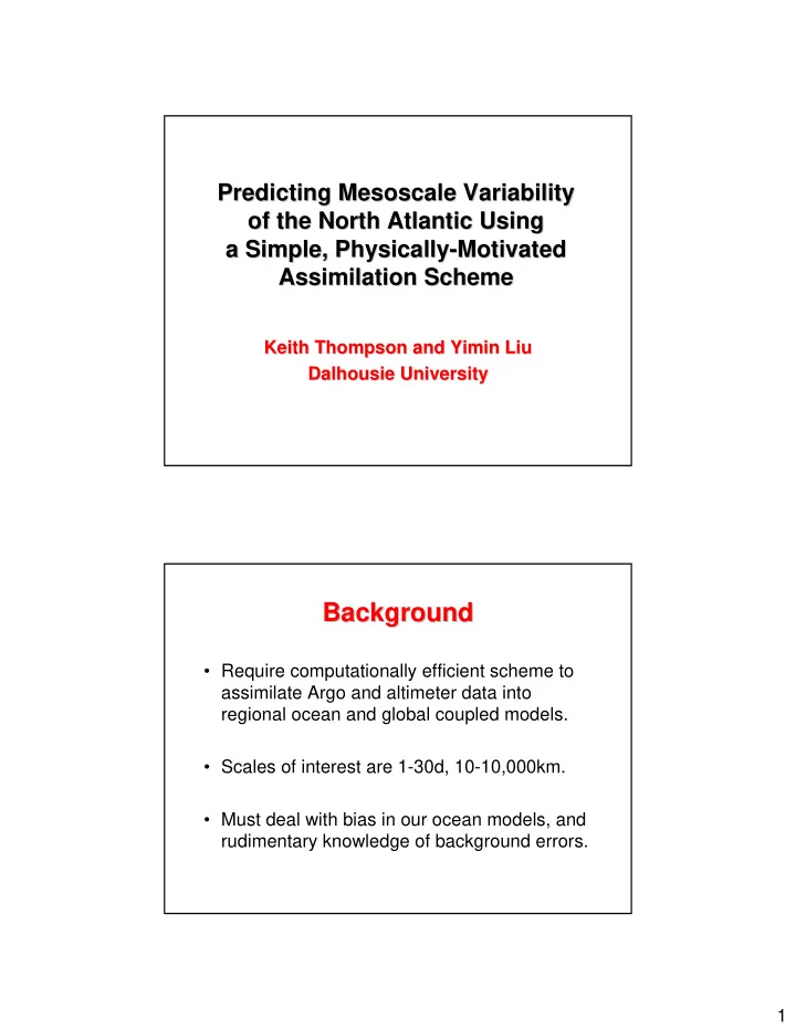
Predicting Mesoscale Mesoscale Variability Variability Predicting of the North Atlantic Using Using of the North Atlantic a Simple, Physically- a Simple, Physically -Motivated Motivated Assimilation Scheme Assimilation Scheme Keith Thompson and Yimin Keith Thompson and Yimin Liu Liu Dalhousie University Dalhousie University Background Background • Require computationally efficient scheme to assimilate Argo and altimeter data into regional ocean and global coupled models. • Scales of interest are 1-30d, 10-10,000km. • Must deal with bias in our ocean models, and rudimentary knowledge of background errors. 1

Observed Sea Level and Observed Sea Level and Dynamic Height From Argo Dynamic Height From Argo • • NW Atlantic NW Atlantic • Anomalies Anomalies • • Colocated Colocated data data • • RL at 1160m RL at 1160m • • Correlation is 0.75, Correlation is 0.75, • slope close to 1 slope close to 1 • Simple physical Simple physical • balance balance Argo Temperature and Salinity Argo Temperature and Salinity • • Scatterplots Scatterplots of T and S of T and S at different depths at different depths • • ~55.2W, 38.4N ~55.2W, 38.4N • Complex, depth • Complex, depth dependent structure dependent structure • • Lines show Lines show Yashayaev Yashayaev climatology climatology • • Shows importance Shows importance of vertical advection in of vertical advection in at depth at depth 2

Modelling Uncertainty Uncertainty Modelling in the Background State Background State in the Motivated by these physical balances, assume T = T b − ∂ T b / ∂ z ξ D + ξ T S = S b − ∂ S b / ∂ z ξ D + ξ S ( ) ∫ η = η b + ∆ ρ ξ D + α T ξ T + α S ξ S dz Builds on: Cooper and Haines (1996), Cooper and Haines (1996), Troccoli Troccoli and Haines and Haines Builds on: (1999), Haines et al. (2006), Ricci et al. (2005), Weaver et (1999), Haines et al. (2006), Ricci et al. (2005), Weaver et al. (2006) al. (2006) Implications for the B Matrix Implications for the B Matrix Assume xi are uncorrelated with separable (x,z) covariance: • • Complex T, S Complex T, S covariance covariance • Depends on Depends on • background background 3

State and Parameter Estimation State and Parameter Estimation Let x and y be true ocean state and observation vectors, and theta a vector of uncertain parameters of covariance of xi. Posterior pdf of state and parameters given observations is p ( x , θ | y ) ∝ p ( y | x ) p ( x | θ ) p ( θ ) Under Gaussian error assumption, maximizing posterior pdf is the same as minimizing L ( x , θ ) ∝ log | B ξξ ( θ ) | + J ( x , θ ) − 2log p ( θ ) J ≡ ( y − Hx ) T R − 1 ( y − Hx )+( x − x b ) T B − 1 ( x − x b ) B ≡ MB ξξ ( θ ) M T Online estimation of theta similar in principle to Dee (1995). Some Details of the Scheme Some Details of the Scheme • Spectral nudging is used to suppress bias in T and S. Online, cheap and necessary. Ensures model and observed climatology match (e.g. western boundary currents separate as observed, mean PE correct) and statistics of variability are reasonable. • Lagrangian interpolation of Argo data to analysis time. • Estimate ocean state daily, and covariance parameters every 2 days. B changes with time (via theta) and background state (via the transformation). 4

North Atlantic Example North Atlantic Example � POP ocean model, 1/3 degree, 23 levels. � Spectrally nudged to Yashayaev monthly climatology. � Daily atmospheric forcing from NCEP reanalysis. � Assimilate Argo and altimeter data, 2003-5. � Vertical gradient of background is linear combination of climatology and forecast. � Uncertain covariance parameters (theta) are horizontal length scales and variance of the xi variables. Typical Snapshot of Sea Level Typical Snapshot of Sea Level 5

Forecast Forecast Skill For Skill For Sea Level Sea Level • • Rms Rms of of o obs bs- -pred pred vs vs lead time lead time Free run Free run • Based on 24 Based on 24 • monthly forecast monthly forecast runs (each 60d) runs (each 60d) Climatology Climatology DA run DA run Forecast Skill for T and S Forecast Skill for T and S 15m 15m 45m 45m 88m 88m 160m 160m 310m 310m 610m 610m tau in days in days tau 6

Summary Summary � New scheme is computationally efficient (adds 30% � New scheme is computationally efficient (adds 30% to run time and memory) and has useful skill. to run time and memory) and has useful skill. � Plan to compare pre � Plan to compare pre- -operational version (with XBT) operational version (with XBT) to existing operational forecast systems (e.g. SEEK). to existing operational forecast systems (e.g. SEEK). � Works because simple physical balances built into B � Works because simple physical balances built into B (which changes with time and background). (which changes with time and background). � Online bias correction is critical for forecasting � Online bias correction is critical for forecasting North Atlantic mesoscale mesoscale. . North Atlantic � Online estimation of B parameters gives scheme � Online estimation of B parameters gives scheme robustness and flexibility. Possible because joint joint robustness and flexibility. Possible because posterior pdf posterior pdf maximized rather than marginal. maximized rather than marginal. Mean Surface Topography From Space Mean Surface Topography From Space ( (Jianliang Jianliang Huang, NRCAN) Huang, NRCAN) MSSH MSSH • GSFC00 GSFC00 • • • Altimeter data 1993 Altimeter data 1993- -9 9 • Multiple satellites Multiple satellites • • • Accuracy O(10cm) in GS Accuracy O(10cm) in GS Geoid Geoid • • GGM02C GGM02C • Regionally enhanced by Regionally enhanced by • blending with terrestrial blending with terrestrial gravity data gravity data 7

MSST of the Spectrally Nudged Model MSST of the Spectrally Nudged Model • • POP POP • Realistic surface fluxes Realistic surface fluxes • • 1991 • 1991- -1999 1999 • • Spectral nudged Spectral nudged • Yashayaev Yashayaev climatology climatology • Similar to classical Similar to classical diagnostic calculation diagnostic calculation based of decades of based of decades of hydrographic data. hydrographic data. Comparing GRACE and Model- Comparing GRACE and Model -Based Based MSST MSST GRACE: Black GRACE: Black Ocean model: Red Red Ocean model: Over whole NA, Over whole NA, rms(error)=7.6cm! rms (error)=7.6cm! 8

Spectral Nudging Gives Realistic Spectral Nudging Gives Realistic Sea Level Variability Sea Level Variability Standard Deviation of Standard Deviation of Standard Deviation of Standard Deviation of Altimeter Data Altimeter Data Model’ Model ’s Sea Level s Sea Level 1993- 1993 -2001 2001 1991- 1991 -9 9 9