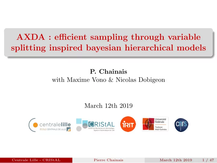
AXDA : efficient sampling through variable splitting inspired - PowerPoint PPT Presentation

AXDA : efficient sampling through variable splitting inspired bayesian hierarchical models P. Chainais with Maxime Vono & Nicolas Dobigeon March 12th 2019 Centrale Lille - CRIStAL Pierre Chainais March 12th 2019 1 / 47

Flight schedule 1 Motivations 2 Splitted Gibbs sampling (SP) 3 Splitted & Augmented Gibbs sampling (SPA) 4 Asymptotically exact data augmentation: AXDA Centrale Lille - CRIStAL Pierre Chainais March 12th 2019 2 / 47

Outline 1 Motivations 2 Splitted Gibbs sampling (SP) 3 Splitted & Augmented Gibbs sampling (SPA) 4 Asymptotically exact data augmentation: AXDA Centrale Lille - CRIStAL Pierre Chainais March 12th 2019 3 / 47

Motivations: applications in image processing Image deblurring Centrale Lille - CRIStAL Pierre Chainais March 12th 2019 4 / 47

Motivations: applications in image processing Image deblurring Centrale Lille - CRIStAL Pierre Chainais March 12th 2019 4 / 47

Motivations: applications in image processing Image inpainting Centrale Lille - CRIStAL Pierre Chainais March 12th 2019 4 / 47

Motivations: applications in image processing Image inpainting Centrale Lille - CRIStAL Pierre Chainais March 12th 2019 4 / 47

Motivations: applications in image processing Confidence intervals 80 70 60 50 40 30 Centrale Lille - CRIStAL Pierre Chainais March 12th 2019 4 / 47

Motivations I have a dream... ◮ solve complex ill-posed inverse problems ◮ big data in large dimensions ◮ excellent performances ◮ fast inference algorithms ◮ credibility intervals with maybe some additional options such as: ◮ parallel distributed computing ◮ privacy preserving Centrale Lille - CRIStAL Pierre Chainais March 12th 2019 5 / 47

Motivations I have a dream... ◮ solve complex ill-posed inverse problems ◮ big data in large dimensions ◮ excellent performances ◮ fast inference algorithms ◮ credibility intervals with maybe some additional options such as: ◮ parallel distributed computing ◮ privacy preserving = ⇒ Bayesian approach + MCMC method! Centrale Lille - CRIStAL Pierre Chainais March 12th 2019 5 / 47

Motivations The optimization-based approach Inverse problems & optimization f ( x ) = f 1 ( x | y ) + f 2 ( x ) = define a cost function : where f 2 is typically ◮ convex (or not) ◮ not differentiable ⇒ proximal operators ◮ a sum of various penalties Solution: proximal operators Centrale Lille - CRIStAL Pierre Chainais March 12th 2019 6 / 47

Motivations The optimization-based approach Inverse problems & optimization f ( x ) = f 1 ( x | y ) + f 2 ( x ) = define a cost function : where f 2 is typically ◮ convex (or not) ◮ not differentiable ⇒ proximal operators ◮ a sum of various penalties Solution: proximal operators and splitting techniques arg min f 1 ( x ) + f 2 ( z ) such that x = z x maybe relaxed to (simplified version of ADMM ) f 1 ( x ) + f 2 ( z ) + α 2 + u T ( x − z ) 2 � x − z � 2 arg min x Centrale Lille - CRIStAL Pierre Chainais March 12th 2019 6 / 47

Motivations The Bayesian approach posterior ∝ likelihood( f 1) × prior( f 2) Inverse problems & Bayes = define a posterior distribution p ( x | y ) = p 1 ( x | y ) · p 2 ( x ) where p 2 is typically ◮ log-concave (or not) ↔ f 2 convex ◮ conjugate ⇒ easy sampling/inference ◮ a combination of various prior Solution: MCMC methods and Gibbs sampling x i ∼ p ( x i | x \ i ) ∀ 1 ≤ i ≤ d Centrale Lille - CRIStAL Pierre Chainais March 12th 2019 7 / 47

Motivations The Bayesian approach posterior ∝ likelihood( f 1) × prior( f 2) Inverse problems & Bayes = define a posterior distribution p ( x | y ) = p 1 ( x | y ) · p 2 ( x ) where p 2 is typically ◮ log-concave (or not) ↔ f 2 convex ◮ conjugate ⇒ easy sampling/inference ◮ a combination of various prior Solution: MCMC methods and Gibbs sampling x i ∼ p ( x i | x \ i ) ∀ 1 ≤ i ≤ d Can we adapt splitting and augmentation from optimization ? � 1 1 � 2 ρ 2 � u − x + z � 2 2 α 2 � u � 2 π ρ ( x , z , u ) ∝ exp − f 1 ( x ) − f 2 ( z ) − 2 − Centrale Lille - CRIStAL Pierre Chainais March 12th 2019 7 / 47

Motivations The Bayesian approach posterior ∝ likelihood( f 1) × prior( f 2) Inverse problems & Bayes = define a posterior distribution p ( x | y ) = p 1 ( x | y ) · p 2 ( x ) Computational motivations: difficult sampling ◮ non-conjugate priors [conj. priors ⇒ easy inference] ◮ rich models: complicated prior distributions ◮ big datasets: expensive likelihood computation Strategy: ❉✐✈✐❞❡✲❚♦✲❈♦♥q✉❡r = ⇒ splitting (SP) and augmentation (SPA) Centrale Lille - CRIStAL Pierre Chainais March 12th 2019 8 / 47

Outline 1 Motivations 2 Splitted Gibbs sampling (SP) 3 Splitted & Augmented Gibbs sampling (SPA) 4 Asymptotically exact data augmentation: AXDA Centrale Lille - CRIStAL Pierre Chainais March 12th 2019 9 / 47

Splitted Gibbs sampling (SP) π ( x ) ∝ exp [ − f 1 ( x ) − f 2 ( x )] ⇓ � 1 � 2 ρ 2 � x − z � 2 π ρ ( x , z ) ∝ exp − f 1 ( x ) − f 2 ( z ) − 2 f 2 z θ x θ z φ ρ f 2 ρ x x f 1 f 1 y y Centrale Lille - CRIStAL Pierre Chainais March 12th 2019 10 / 47

Splitted Gibbs sampling (SP) π ( x ) ∝ exp [ − f 1 ( x ) − f 2 ( x )] ⇓ π ρ ( x , z ) ∝ exp [ − f 1 ( x ) − f 2 ( z ) − φ ρ ( x , z )] f 2 z θ x θ z φ ρ f 2 ρ x x f 1 f 1 y y Centrale Lille - CRIStAL Pierre Chainais March 12th 2019 10 / 47

Splitted Gibbs sampling (SP): Theorem 1 Consider the marginal of x under π ρ : � � p ρ ( x ) = R d π ρ ( x , z )d z ∝ R d exp [ − f 1 ( x ) − f 2 ( z ) − φ ρ ( x , z )] d z . Theorem Assume that in the limiting case ρ → 0 , φ ρ is such that exp ( − φ ρ ( x , z )) R d exp ( − φ ρ ( x , z )) d x − ρ → 0 δ x ( z ) − − → � Then p ρ coincides with π when ρ → 0 , that is � p ρ − π � TV − ρ → 0 0 − − → Centrale Lille - CRIStAL Pierre Chainais March 12th 2019 11 / 47

Splitted Gibbs sampling (SP): marginal distributions Full conditional distributions under the split distribution π ρ : π ρ ( x | z ) ∝ exp ( − f 1 ( x ) − φ ρ ( x , z )) π ρ ( z | x ) ∝ exp ( − f 2 ( z ) − φ ρ ( x , z )) . Note that f 1 and f 2 are now separated in 2 distinct distributions Centrale Lille - CRIStAL Pierre Chainais March 12th 2019 12 / 47

Splitted Gibbs sampling (SP): marginal distributions Full conditional distributions under the split distribution π ρ : � 1 � 2 ρ 2 � x − z � 2 π ρ ( x | z ) ∝ exp − f 1 ( x ) − 2 � 1 � 2 ρ 2 � x − z � 2 π ρ ( z | x ) ∝ exp − f 2 ( z ) − . 2 Note that f 1 and f 2 are now separated in 2 distinct distributions State of the art sampling methods: ◮ P-MYULA = proximal MCMC, (Pereyra 2016; Durmus et al. 2018) ◮ Fourier or Aux-V1 or E-PO for Gaussian variables ◮ ... Centrale Lille - CRIStAL Pierre Chainais March 12th 2019 12 / 47

Splitted Gibbs sampling (SP): inverse problems Linear Gaussian inverse problems y = Px + n , � 0 d , σ 2 I d � where P = damaging operator and n ∼ N = noise. 1  2 σ 2 � y − Px � 2 ∀ x ∈ R d , f 1 ( x ) =  2 f 2 ( x ) = τψ ( x ) , τ > 0 .  Then the SP conditional distributions are: µ x , Q x − 1 � � π ρ ( x | z ) = N � 1 � 2 ρ 2 � z − x � 2 π ρ ( z | x ) ∝ exp − τψ ( z ) − , 2 Centrale Lille - CRIStAL Pierre Chainais March 12th 2019 13 / 47

Splitted Gibbs sampling (SP): efficient sampling Linear Gaussian inverse problems µ x , Q x − 1 � � π ρ ( x | z ) = N � � 1 2 ρ 2 � z − x � 2 π ρ ( z | x ) ∝ exp − τψ ( z ) − , 2 Examples: ◮ Convex non-smooth ψ ( x ) = TV , ℓ 1 sparsity... ⇒ proximal MCMC ◮ Tikhonov regularization ψ ( z ) = � Qz � 2 2 ⇒ Gaussian variables (e.g. P or Q diagonalizable in Fourier → E-PO) Centrale Lille - CRIStAL Pierre Chainais March 12th 2019 14 / 47

Splitted Gibbs sampling (SP): TV deblurring Linear Gaussian inverse problems Posterior distribution � � − 1 2 σ 2 � Px − y � 2 p ( x | y ) ∝ exp 2 − β TV( x ) where P = damaging operator (blur, binary mask...) and � � � TV( x ) = � ( ∇ x ) i,j � � � 2 1 ≤ i,j ≤ N Direct sampling is challenging 1 generally high dimension of the image, 2 non-conjugacy of the TV-based prior, 3 non-differentiability of g ( � = Hamiltonian Monte Carlo algorithms) Centrale Lille - CRIStAL Pierre Chainais March 12th 2019 15 / 47

Splitted Gibbs sampling (SP): TV deblurring Linear Gaussian inverse problems Centrale Lille - CRIStAL Pierre Chainais March 12th 2019 16 / 47

Splitted Gibbs sampling (SP): TV deblurring Linear Gaussian inverse problems Centrale Lille - CRIStAL Pierre Chainais March 12th 2019 16 / 47

Splitted Gibbs sampling (SP): TV deblurring Linear Gaussian inverse problems 65 60 55 50 45 40 35 30 25 20 Centrale Lille - CRIStAL Pierre Chainais March 12th 2019 16 / 47

Splitted Gibbs sampling (SP): TV deblurring Linear Gaussian inverse problems SALSA FISTA SGS P-MYULA time (s) 1 10 470 3600 time ( × var. split.) 1 10 1 7.7 ∼ 10 4 10 5 nb. iterations 22 214 SNR (dB) 17.87 17.86 18.36 17.97 Rk : ρ 2 = 9 Centrale Lille - CRIStAL Pierre Chainais March 12th 2019 17 / 47