Automata-theoretic analysis of hybrid systems Madhavan Mukund SPIC - PDF document
Automata-theoretic analysis of hybrid systems Madhavan Mukund SPIC Mathematical Institute 92, G N Chetty Road Chennai 600 017, India Email: madhavan@smi.ernet.in URL: http://www.smi.ernet.in/~madhavan Tutorial at BRNS Workshop on Verification
Automata-theoretic analysis of hybrid systems Madhavan Mukund SPIC Mathematical Institute 92, G N Chetty Road Chennai 600 017, India Email: madhavan@smi.ernet.in URL: http://www.smi.ernet.in/~madhavan Tutorial at BRNS Workshop on Verification of Digital and Hybrid Systems, January 7–11, 1999, TIFR, Mumbai, India.
What is a hybrid system? • Digital system which reads and reacts to analog environmental parameters such as time, position, temperature . . . • Examples: – Controllers for cars, aircraft, manufacturing plants – Medical equipment – Robots • Extension of finite-state automata with ana- log inputs— hybrid automata . 2
Example: A temperature controller (thermostat) • Heater may be off or on . • If heater is off , temperature drops exponentially — T ( t ) = T init e − kt • If heater is on , temperature rises exponentially — T ( t ) = T init e − kt + h (1 − e − kt ) • Heater switches between on and off when temperature crosses threshold values. Typical question: Show that heater is on for less than 50% of the first 60 units of time. 3
on x = 2 ∧ y = 0 ∧ z = 0 1 ≤ x ≤ 3 ∧ ˙ x = 5 − x ∧ ˙ y = 1 ∧ ˙ z = 1 turnoff x = 3 ∧ stable ( x, y, z ) turnon x = 1 ∧ stable ( x, y, z ) off 1 ≤ x ≤ 3 ∧ ˙ x = − x ∧ ˙ y = 0 ∧ ˙ z = 1 4 A thermostat
Hybrid automata A hybrid automaton consists of: • A finite set V of control modes — i.e., states, in the sense of automata theory. In the example, V = { on , off } . • A finite set E of control switches — i.e., transitions, in the sense of automata the- ory. In the example, E = { (on , off) , (off , on) } . ( V, E ) defines a directed graph, as usual. • A set X of variables taking values over R . In the example, X = { x, y, z } . For each variable x , x denotes the first ˙ derivative of x with respect to time. This is called the flow of x . 5
Labels on control modes: • Control modes labelled by initial condition init ( v ) and flow condition flow ( v ) — predicates over X ∪ ˙ X . In the example: – init (on) : x = 2 ∧ y = 0 ∧ z = 0 – flow (on) : 1 ≤ x ≤ 3 ∧ x = 5 − x ∧ ˙ y = 1 ∧ ˙ z = 1 ˙ • Initial conditions marked on incoming arcs with no source state. Initial condition false is not marked — for instance, init (off). • Flow condition flow ( v ) constrains flows in the control mode v — for instance, x = 5 − x . ˙ • Flow conditions implicitly include invariants — for instance, 1 ≤ x ≤ 3. 6
Labels on control switches: • Control switches ( v, v ′ ) labelled by jump condition jump ( v, v ′ ) — predicate over X, X ′ , ˙ X ′ . X, ˙ Jump condition relates values of variables before and after the transition — x ′ and ˙ x ′ denote values of x and ˙ x after the transi- tion. Example: jump (on , off) : x = 3 ∧ stable ( x, y, z ) where stable ( x ) abbreviates x ′ = x . • Control switches also labelled by events — used for synchronization of parallel compo- nents. Example: (off , on) is labelled by the event turnon . 7
Special types of variables • A clock is a variable with constant flow 1, which is either stable or reset to 0 on each control switch. In the thermostat automaton, z is a clock. • A stopwatch is a variable which can have flows 0 or 1, which is either stable or reset to 0 on each control switch. In the thermostat automaton, y is a stop- watch which measures how much time the system spends in control mode on . • Show that heater is on for less than 50% of the first 60 units of time. is equivalent to proving that ( z = 60) implies y ≤ z/ 2 8
Controller for a railway level crossing When the train is far from the gate it moves at 48 to 52 m/s. At 1000 m from the gate is a sensor. After passing the sensor, the train slows down to 40 to 52 m/s. After sensing the train, the controller requires upto 5 secs to start lowering the gate. The gate moves at 20 deg/s. At 100 m past the gate, there is a second sen- sor. Once the train passes this sensor, the controller requires upto 5 secs to start raising the gate. The gate again moves at 20 deg/s. Consecutive trains are at least 1500 m apart. 9
far near app 1000 ≤ x 0 ≤ x ≤ 1000 x = 1000 48 ≤ − ˙ x ≤ 52 40 ≤ − ˙ x ≤ 52 x = 100 → exit x ′ ≥ 1500 x = 0 past Train 0 ≤ x ≤ 1000 40 ≤ − ˙ x ≤ 52 Controller app exit app exit idle z ′ = 0 z ′ = 0 0 ≤ z ≤ 5 0 ≤ z ≤ 5 z = 0 ˙ z = 1 ˙ z = 1 ˙ lower raise z ′ = 0 app exit 10
open up raise raise y = 90 0 ≤ y ≤ 90 y = 90 y = 0 ˙ y = 20 ˙ lower lower raise raise down closed 0 ≤ y ≤ 90 y = 0 y = 0 y = − 20 ˙ y = 0 ˙ lower lower Gate 11
Configurations • A configuration is a triple ( v, a , ˙ a ) where a is a point in R n and ˙ a is a vector of trajectories, also in R n . • Let ϕ be a predicate over X ∪ ˙ X . The models of ϕ , [ [ ϕ ] ], is defined as: is true when X ← a , ˙ [ [ ϕ ] ] = {� a , ˙ a � | ϕ X ← ˙ a } . • The configuration ( v, a , ˙ a ) is admissible if � a , ˙ a � belongs to [ [ flow ( v )] ]. • The configuration ( v, a , ˙ a ) is initial if � a , ˙ a � belongs to [ [ init ( v )] ]. 12
Timed Transition Systems TTS = ( Q, Q i , Σ , − → ) • Q a set of states with initial states Q i ⊆ Q . • Set of actions Σ, includes silent action τ . • Labelled transition relation − → ⊆ Q × (Σ ∪ R ≥ 0 ) × Q . a → q ′ , a ∈ Σ. Jump transition: q − If a = τ , the transition is silent . δ Flow transition: q − → q , δ ∈ R ≥ 0 . 13
Hybrid automaton Timed transition system = ⇒ TTS A = ( Q, Q i , Σ , − A → ) Q : admissible configurations of A Q i : initial configurations of A Σ : events of A → : moves of the following form: − σ a ′ ) → ( v ′ , a ′ , ˙ Jump : ( v, a , ˙ a ) − – σ is the event label on edge ( v, v ′ ) a ′ � belongs to [ a , a ′ , ˙ [ jump ( v, v ′ )] – � a , ˙ ] δ → ( v, a ′ , ˙ a ′ ) Flow : ( v, a , ˙ a ) − – δ = 0, a = a ′ and ˙ a ′ , a = ˙ or – there exists f : [0 , δ ] → R n , f is continuously differentiable, � f (0) , ˙ f (0) � = � a , ˙ a � , a ′ � , f ( δ ) � = � a ′ , ˙ � f ( δ ) , ˙ and � f ( t ) , ˙ f ( t ) � in [ [ flow ( v )] ] for all t ∈ [0 , δ ]. 14
Reachability • A trajectory of automaton A is a finite a n − 1 a 0 a 1 path s 0 − → s 1 − → · · · − → s n in TTS A , where s 0 is an initial state and each move is permitted by − → . State s is reachable if there is a trajectory from an initial state which ends in s . Question: Given an automaton A and a state s , is s reachable in A ? Non-emptiness: Infinite behaviours a 0 a 1 • An infinite path s 0 − → s 1 − → · · · in TTS A diverges if the time elapsed in flow transi- tions tends to ∞ . Question: Given an automaton A , does TTS A admit at least one divergent infinite path? 15
Reachability and non-emptiness are decidable for very restricted classes of hybrid systems. A timed automaton is a hybrid system where • Every variable is a clock. • Every jump condition is simple — comparison of variables to constants or the difference of two variables to a constant. For example, x ≤ 5 ∧ y − z ≥ 3 ∧ x ′ = 7. Theorem Reachability and non-emptiness are decidable (PSPACE-complete) for timed au- tomata. 16
A multirate timed system extends timed au- tomata with variables with arbitrary constant slope. Reachability is undecidable for 2- Theorem rate timed systems. Reduction of halting problem for non- Proof deterministic 2-counter machines. Use accurate clocks with slope 1 and skewed clocks with slope 2. Use an accurate clock y to mark off time seg- ments of unit length. 1 y t 17
Counter value n ⇔ Accurate clock value x = 1 2 n To reproduce x ( t ) at x ( t +1), reset when x = 1. 1 x 0 t +1 t To increment x : 1 x z z ′ 0 x = 1 1 x = 2 n 2 n +1 To decrement x : 1 x z z ′ 0 1 x = 1 x = 2 n − 1 2 n 18
Rectangular automata • ˙ x can vary within a range [ min , max ]. Can model drifting clocks . • Values of variables with different flows are never compared. • Whenever the flow constraint of a variable changes, the variable is reset. Reachability is decidable for rect- Theorem angular automata. Theorem Reachability is undecidable if either the second or the third constraint is violated. 19
Linear hybrid automata • A linear predicate over X built out of atomic predicates of the form Σ i a i x i op c , where op is a relational operator. If all the a i ’s are rational, this is called a rational linear predicate . • In a linear hybrid automaton , all initial, jump and flow conditions are written using linear predicates such that variables from X and ˙ X never appear together in an atomic predicate. For instance, x + 2 ˙ y ≤ 7 or x = − ˙ x is not allowed, but x ≤ 7 ∧ 3 ˙ x + 2 ˙ y = 8 is allowed. 20
Linear regions • A region is a set of configurations of A . • A region R is linear if there is a linear pred- icate ϕ v for each control mode v such that R = � v ∈ V { v } × [ [ ϕ v ] ]. Example: Let A be a linear hybrid automa- ton and let TTS A be its timed transition system. Then, Q , Q i are linear regions. • Let R be a region. post ( R ) = { s 2 | ∃ s 1 ∈ R.s 1 − → s 2 } . pre ( R ) = { s 1 | ∃ s 2 ∈ R.s 1 − → s 2 } . 21
Recommend
More recommend
Explore More Topics
Stay informed with curated content and fresh updates.
