Asymptotic expansions for the profile of random trees 80000 60000 - - PowerPoint PPT Presentation

Asymptotic expansions for the profile of random trees

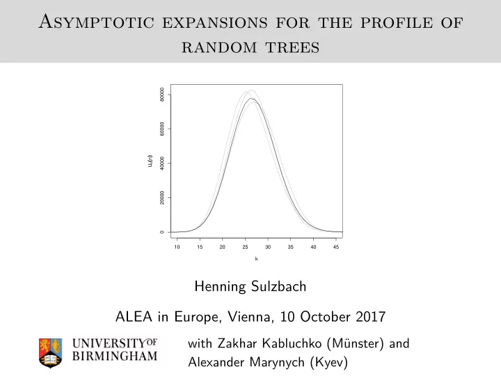
10 15 20 25 30 35 40 45 20000 40000 60000 80000 k Uk(n)

Henning Sulzbach ALEA in Europe, Vienna, 10 October 2017

with Zakhar Kabluchko (Münster) and Alexander Marynych (Kyev)

Trees of interest

• data structures
• analysis of algo.
• real-world networks

Comparison-based: binary (m-ary) search trees, random recursive trees, preferential attachment trees Multidimensional: quadtrees, K-d trees Digital: digital search trees, tries Trees are flat (i.e. logarithmic) and wide.

Quantities of interest

Global quantities:

• typical depths and distances,
• maximal depths and distances,
• total pathlength (sum over all node depths),
• mode and width.

Local quantities:

• degree distribution,
• fringe subtrees.

Put simply, the profile.

Outline

• 1. One-split branching random walks
• 2. Profile of binary search trees: a summary
• 3. Main result: an asymptotic profile expansion

Outline

• 1. One-split branching random walks
• 2. Profile of binary search trees: a summary
• 3. Main result: an asymptotic profile expansion

The binary search tree

Input: numbers 0.6, 0.9, 0.3, 0.7, 0.5, 0.8, 0.1, 0.2

The binary search tree

Input: numbers 0.6, 0.9, 0.3, 0.7, 0.5, 0.8, 0.1, 0.2

.6

The binary search tree

Input: numbers 0.6, 0.9, 0.3, 0.7, 0.5, 0.8, 0.1, 0.2

.6 .9

The binary search tree

Input: numbers 0.6, 0.9, 0.3, 0.7, 0.5, 0.8, 0.1, 0.2

.6 .9 .3

The binary search tree

Input: numbers 0.6, 0.9, 0.3, 0.7, 0.5, 0.8, 0.1, 0.2

.6 .9 .7 .3

The binary search tree

Input: numbers 0.6, 0.9, 0.3, 0.7, 0.5, 0.8, 0.1, 0.2

.6 .9 .7 .3 .5

The binary search tree

Input: numbers 0.6, 0.9, 0.3, 0.7, 0.5, 0.8, 0.1, 0.2

.6 .9 .7 .8 .3 .5

The binary search tree

Input: numbers 0.6, 0.9, 0.3, 0.7, 0.5, 0.8, 0.1, 0.2

.6 .9 .7 .8 .3 .5 .1

The binary search tree

Input: numbers 0.6, 0.9, 0.3, 0.7, 0.5, 0.8, 0.1, 0.2

.6 .9 .7 .8 .3 .5 .2 .1

The binary search tree

Input: numbers 0.6, 0.9, 0.3, 0.7, 0.5, 0.8, 0.1, 0.2

.6 .9 .7 .8 .3 .5 .2 .1

Model: Use iid unif[0, 1] random variables U1, U2, U3, . . .

The binary search tree - a Markov chain

The binary search tree - a Markov chain

The binary search tree - a Markov chain

The binary search tree - a Markov chain

The binary search tree - a Markov chain

The binary search tree - a Markov chain

The binary search tree - a Markov chain

The binary search tree - a Markov chain

The binary search tree - a Markov chain

The binary search tree - a Markov chain

The binary search tree - a Markov chain

Xn(k) = #{nodes with depth k}, k ≥ 0, Un(k) = #{boxes with depth k}, k ≥ 0.

The binary search tree - a Markov chain

Xn = (1, 2, 4, 6, 5, 0, 0, . . .) Un = (0, 0, 0, 2, 7, 10, 0, . . .)

The binary search tree - three simulations

20 30 40 50 60 70 1 2 3 4 5 6 7 108

n = 1010, heights between 87 and 91.

The binary search tree - Logplot

10 20 30 40 50 60 70 80 90 100 0.1 0.2 0.3 0.4 0.5 0.6 0.7 0.8 0.9 1

n = 1010, heights between 87 and 91.

The random recursive tree

1/2

The random recursive tree

1/2 1/2

The random recursive tree

1/3 1/3 1/3

The random recursive tree

1/4 1/4 1/4 1/4 1/4

The random recursive tree

1/4 1/4

The random recursive tree

1/4 1/4

The random recursive tree

The random recursive tree - three simulations

n = 1010, heights between 57 and 62.

The plane-oriented recursive tree

The plane-oriented recursive tree

The plane-oriented recursive tree

The plane-oriented recursive tree

The plane-oriented recursive tree

The plane-oriented recursive tree

weight of v: 1 + dv degree profile: j−2

One-split branching random walks

Input: random point process ζ on Z

One-split branching random walks

Input: random point process ζ on Z Zn(k) : # of particles at k at time n Z0(k) = δ0,k

• 3
• 2
• 1

1 2 3 4

Z0 = (. . . , 0, 0, 1∗, 0, 0, . . .) Assumptions:

• 1 ≤ ζ(Z) ≤ C, P (ζ(Z) > 1) > 0 and ζ has bounded support,
• P (ζ(cZ) < ζ(Z)) > 0 for all c ≥ 2. (wlog)

One-split branching random walks

Input: random point process ζ on Z Zn(k) : # of particles at k at time n Z0(k) = δ0,k

• 3
• 2
• 1

1 2 3 4

Z0 = (. . . , 0, 0, 1∗, 0, 0, . . .) Assumptions:

• 1 ≤ ζ(Z) ≤ C, P (ζ(Z) > 1) > 0 and ζ has bounded support,
• P (ζ(cZ) < ζ(Z)) > 0 for all c ≥ 2. (wlog)

One-split branching random walks

Input: random point process ζ on Z Zn(k) : # of particles at k at time n Z0(k) = δ0,k

• 3
• 2
• 1

1 2 3 4

ζ = (. . . , 0, 1, 0∗, 0, 1, 1, 0 . . .) Z0 = (. . . , 0, 0, 1∗, 0, 0, . . .) Assumptions:

• 1 ≤ ζ(Z) ≤ C, P (ζ(Z) > 1) > 0 and ζ has bounded support,
• P (ζ(cZ) < ζ(Z)) > 0 for all c ≥ 2. (wlog)

One-split branching random walks

Input: random point process ζ on Z Zn(k) : # of particles at k at time n Z0(k) = δ0,k

• 3
• 2
• 1

1 2 3 4

Z1 = (. . . , 0, 1, 0∗, 0, 1, 1, 0, . . .) Assumptions:

• 1 ≤ ζ(Z) ≤ C, P (ζ(Z) > 1) > 0 and ζ has bounded support,
• P (ζ(cZ) < ζ(Z)) > 0 for all c ≥ 2. (wlog)

One-split branching random walks

Input: random point process ζ on Z Zn(k) : # of particles at k at time n Z0(k) = δ0,k

• 3
• 2
• 1

1 2 3 4

Z1 = (. . . , 0, 1, 0∗, 0, 1, 1, 0, . . .) Assumptions:

• 1 ≤ ζ(Z) ≤ C, P (ζ(Z) > 1) > 0 and ζ has bounded support,
• P (ζ(cZ) < ζ(Z)) > 0 for all c ≥ 2. (wlog)

One-split branching random walks

Input: random point process ζ on Z Zn(k) : # of particles at k at time n Z0(k) = δ0,k

• 3
• 2
• 1

1 2 3 4

ζ = (. . . , 0, 1, 0, 0∗, 0, 1, 0, . . .) Z1 = (. . . , 0, 1, 0∗, 0, 1, 1, 0, . . .) Assumptions:

• 1 ≤ ζ(Z) ≤ C, P (ζ(Z) > 1) > 0 and ζ has bounded support,
• P (ζ(cZ) < ζ(Z)) > 0 for all c ≥ 2. (wlog)

One-split branching random walks

Input: random point process ζ on Z Zn(k) : # of particles at k at time n Z0(k) = δ0,k

• 3
• 2
• 1

1 2 3 4

Z2 = (. . . , 0, 1, 1∗, 0, 0, 1, 1, 0 . . .) Assumptions:

• 1 ≤ ζ(Z) ≤ C, P (ζ(Z) > 1) > 0 and ζ has bounded support,
• P (ζ(cZ) < ζ(Z)) > 0 for all c ≥ 2. (wlog)

One-split branching random walks

Input: random point process ζ on Z Zn(k) : # of particles at k at time n Z0(k) = δ0,k

• 3
• 2
• 1

1 2 3 4

Z2 = (. . . , 0, 1, 1∗, 0, 0, 1, 1, 0 . . .) Assumptions:

• 1 ≤ ζ(Z) ≤ C, P (ζ(Z) > 1) > 0 and ζ has bounded support,
• P (ζ(cZ) < ζ(Z)) > 0 for all c ≥ 2. (wlog)

One-split branching random walks

Input: random point process ζ on Z Zn(k) : # of particles at k at time n Z0(k) = δ0,k

• 3
• 2
• 1

1 2 3 4

ζ = (. . . , 0, 1, 0∗, 0, 0, 1, 0 . . .) Z2 = (. . . , 0, 1, 1∗, 0, 0, 1, 1, 0 . . .) Assumptions:

• 1 ≤ ζ(Z) ≤ C, P (ζ(Z) > 1) > 0 and ζ has bounded support,
• P (ζ(cZ) < ζ(Z)) > 0 for all c ≥ 2. (wlog)

One-split branching random walks

Input: random point process ζ on Z Zn(k) : # of particles at k at time n Z0(k) = δ0,k

• 3
• 2
• 1

1 2 3 4

One-split branching random walks

Input: random point process ζ on Z Zn(k) : # of particles at k at time n Z0(k) = δ0,k

• 3
• 2
• 1

1 2 3 4

Z3 = (. . . , 0, 2, 0∗, 0, 0, 2, 1, 0 . . .) Assumptions:

• 1 ≤ ζ(Z) ≤ C, P (ζ(Z) > 1) > 0 and ζ has bounded support,
• P (ζ(cZ) < ζ(Z)) > 0 for all c ≥ 2. (wlog)

One-split branching random walks

BST: ζ = (. . . , 0, 0∗, 2, 0, . . .) = 2δ1 RRT: ζ = (. . . , 0, 1∗, 1, 0, . . .) = δ0 + δ1 PORT: ζ = (. . . , 0, 2∗, 1, 0, . . .) = 2δ0 +δ1 Note: ζ is deterministic.

Outline

• 1. One-split branching random walks
• 2. Profile of binary search trees: a summary
• 3. Main result: an asymptotic profile expansion

Binary search tree - a rough picture

x 1 η 0 α− α+ 2 η(x) = x − x log(x/2) − 1, α− = 0.37 . . . , α+ = 4.31 . . . , η(2) = 1. For k = α log n + o(log n), as n → ∞, Un(k) = nη(α)+o(1), α− < α < α+. As n → ∞, Dn − 2 log n √2 log n

d

→ N and Height ∼ α+ log n, Fill-up level ∼ α− log n.

Devroye ’86 -’88

Profile - central regime

Recall: As n → ∞, Dn − 2 log n √2 log n

d

→ N.

2√2 log n 2 log n k

n

√

4π log n

Un(k)

With xn(k) := k − 2 log n √2 log n , uniformly over k ∈ N, almost surely and in mean, Un(k) = n √2π · 2 log n · e− 1

2 x2 n (k) · (1 + o(1)) .

Hwang ’95, Chauvin, Drmota and Jabbour-Hattab ’01

Width and mode

20 30 40 50 60 70 1 2 3 4 5 6 7 108

Wn := max{Un(k) : k ≥ 1} mn := max{k : Un(k) = Wn} Wn = n √4π log n · (1 + o(1)) Open: Limit theorem for Wn The sequence (mn − 2 log n)n≥1 is tight.

Devroye and Hwang ’06

Open: Limit theorem for mn − 2 log n

Profile - limit theorem

Theorem (Hwang ’95)

For C > 0, uniformly in 0 ≤ k ≤ C log n, as n → ∞, E [Un(k)] ∼ 1 Γ(αk) · √2παk · nη(αk) √log n, αk = k log n.

Theorem (Chauvin, Klein, Marckert and Rouault ’05)

There exists a random analytic function X on a complex domain G with (α−, α+) ⊆ G with E [X(α)] = 1 and X > 0 on (α−, α+): sup

αk∈(α−,α+)

• Un(k)

E [Un(k)] − X(αk)

• a.s.

− → 0.

The special regimes

The limit X(α) is random if α / ∈ {1, 2}.

Theorem (Fuchs, Hwang and Neininger ’06)

Let c ∈ {1, 2}. For k = c log n + cn with cn = o(log n) and |cn| → ∞, we have Un(k)∗

d

− → (X ′(c))∗. (Un(k)∗)n≥1 does not converge in distribution if cn = O(1). For Pn :=

k k · Un(k):

P∗

n a.s.

− → (X ′(2))∗.

Régnier ’89, Rösler ’91

The internal profile

x α · log 2

almost full

1 η 0 α− α+ 1 2 Xn(k) = nη(α)+o(1), 1 < α < α+ 2k − Xn(k) = nη(α)+o(1), α− < α < 1. Analogous mean expansions and limit theorems for Xn(k) for k log n ∈ (1, α+), 2k − Xn(k) for k log n ∈ (α−, 1).

Hwang ’95, Chauvin, Drmota and Jabbour-Hattab ’01

Techniques and references

FORWARD

• Jabbour-Hattab ’01
• Chauvin, Drmota and

Jabbour-Hattab ’01

• Chauvin, Klein, Marckert

and Rouault ’05

• Katona ’05
• Labarbe ’08
• Schopp ’10
• Mailler and Marckert ’17

BACKWARD

• Drmota and Hwang ’04
• Drmota and Hwang ’05
• Fuchs, Hwang and

Neininger ’06

• Devroye and Hwang ’06
• Hwang ’07
• Drmota, Janson

Neininger ’08

Outline

• 1. One-split branching random walks
• 2. Profile of binary search trees: a summary
• 3. Main result: an asymptotic profile expansion

Classical Chebyshev-Edgeworth-Cramér expansion

Let Z1, Z2, . . . be iid integer random variables with

• E
• etZ1
• < ∞ in a neighbourhood of 0,
• E [Z1] = 0, Var(Z1) = 1,
• Z1 is not concentrated on a non-trivial sublattice.

Then, with Sn = Z1 + · · · + Zn, xn(k) =

k √n and r ∈ N0:

n

r+1 2 sup

k∈Z

• P (Sn = k) − e− 1

2 x2 n (k)

√ 2πn

r

• s=0

Qs(xn(k)) ns/2

• → 0,

where Qs is a polynomial of degree 3s expressed through the cumulants κ2, . . . , κs+2. Q0 = 1 and Q1(x) = κ3 6 He3(x), Q2(x) = κ4 24He4(x) + κ2

3

72He6(x).

Profile expansion for the binary search tree

Theorem (Kabluchko, Marynych and S. ’16)

Let Un(k) be the external profile of a sequence of random binary search trees. Set

xn(k) = xn(k; α) = k − α log n √α log n , αk = k log n.

Fix r ≥ 0, K ⊆ (α−, α+) compact. Uniformly in k ∈ N and α ∈ K

(log n)

r+1 2

• Un(k)

nα−1−αk·log α/2 − e− 1

2 x2 n (k)

√2π · α log n

r

• s=0

Fs(xn(k); α) (log n)s/2

• a.s.

− → 0,

where Fs(x; α) is a polynomial in x of degree 3s whose coefficients are linear combinations of X(α), . . . , X (s)(α).

Profile expansion for the binary search tree

(log n)

r+1 2

• Un(k)

nα−1−αk·log α/2 − e− 1

2 x2 n (k)

√2π · α log n

r

• s=0

Fs(xn(k); α) (log n)s/2

• a.s.

− → 0,

where F0(x; α) = X(α) and

F1(x; α) = X ′(α) √α x + X(α) 6√α He3(x), F2(x; α) = X ′′(α) 2α He2(x) + X(α) 24α + X ′(α) 6α

• He4(x)

+ X(α) 72α He6(x), and the first Hermite polynomials are He2(x) = x2 − 1, He3(x) = x3 − 3x, He4(x) = x4 − 6x2 + 3, He6(x) = x6 − 15x4 + 45x2 − 15.

External BST profile - central regime

Recall: For k = 2 log n + cn and cn = O(1), the sequence

• Un(k) − E [Un(k)]
• Var(Un(k))
• n≥1

does not converge in distribution.

Corollary (Kabluchko, Marynych and S. ’16)

Let k = ⌊2 log n⌋ + a with a ∈ Z. Then, as n → ∞, (log n)3/2 n (Un(k) − E [Un(k)]) − X ′(2) 4√π ({2 log n} + a + 1/2)

a.s.

− → −χ − E [χ] 8√π , where {x} := x − ⌊x⌋ and χ = X ′′(2) − X ′(2)2.

External BST profile - mode

Recall: mn − 2 log n, n ≥ 1 is a tight sequence.

Corollary (Kabluchko, Marynych and S. ’16)

For all n sufficiently large, mn takes its value(s) in the set {⌊2 log n + X ′(2) − 1/2⌋, ⌈2 log n + X ′(2) − 1/2⌉}. For a set of asymptotic frequency 1, mn is equal to the integer closest to 2 log n + X ′(2) − 1/2.

The width - more periodicities

Recall: Wn ∼

n

√

4π log n almost surely.

Corollary (Kabluchko, Marynych and S. ’16)

Let W n := 4 log n

• 1 −

√4π log nWn n

• .

Then, W n − θ2

n a.s.

− → χ − 1 12, where χ = X ′′(2) − X ′(2)2, θn = min

k∈Z

• 2 log n + X ′(2) − 1/2 − k
• .

Outline

• 1. One-split branching random walks
• 2. Profile of binary search trees: a summary
• 3. Main result: an asymptotic profile expansion

Discussion - the proof

Fourier inversion using Wn(λ) =

• k∈N

Un(k) · eλk, λ ∈ C. Then, E [Wn(λ)] = n2eλ−1 Γ(2eλ) · (1 + o(1)), ℜ(λ) > 0.

Brown and Shubert ’84, Jabbour-Hattab ’01

Theorem (Chauvin, Klein, Marckert, Rouault ’05)

There exists a complex domain G with (log α−

2 , log α+ 2 ) ⊆ G such

that, almost surely, uniformly on compact sets K ⊆ G with polynomial rate of convergence, Wn(λ) E [Wn(λ)] → W (λ), and X(α) = W (log α

2 ). Biggins ’77, ’92

Discussion - generalisations

Analogous expansions for

• general profiles An(k), k ∈ Z, n ≥ 1 with

e−wn·ϕ(λ) ·

• k∈Z

An(k) · eλk → Ψ(λ), with an analytic function Ψ, where

• wn → ∞,
• ϕ is strictly convex on R,
• the convergence is exponential in wn on compact subsets of a

domain close to the real axis,

• e−wn·ϕ(θ) ·

k∈Z An(k) · e(θ+iη)k → 0 for ε < |η| < π with

exponential rate of convergence.

• the profile of one-split branching random walks,
• the expected profile if ζ(Z) is deterministic,
• standard lattice BRWs

Grübel and Kabluchko ’15

Summary and conclusion

• full uniform asymptotic profile expansion,
• precise information on occupation numbers, mode and width

can be extracted almost automatically,

• extends to more general profiles An(k), k ∈ Z, n ≥ 1 upon

controlling

∞

• k∈Z

An(k) · eλk.

• martingale-free trees? Split trees?

THANK YOU