Assessing Structural VARs by Lawrence J. Christiano, Martin - PowerPoint PPT Presentation
... Assessing Structural VARs by Lawrence J. Christiano, Martin Eichenbaum and Robert Vigfusson Minneapolis, August 2005 1 Background In Principle, Impulse Response Functions from SVARs are useful as a guide to constructing and
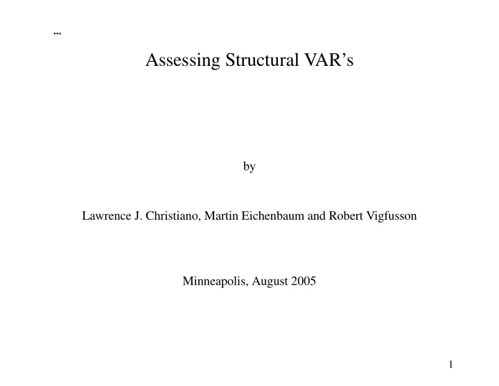
... Assessing Structural VAR’s by Lawrence J. Christiano, Martin Eichenbaum and Robert Vigfusson Minneapolis, August 2005 1
Background • In Principle, Impulse Response Functions from SVARs are useful as a guide to constructing and evaluating Dynamic Stochastic General Equilibrium (DSGE) models. • To be useful in practice, estimators of response functions must have good sampling properties. 2
What We Do • Investigate the Sampling Properties of SVARs, When Data are Generated by Estimated DSGE Models. – Bias Properties of Impulse Response Function Estimators ∗ Bias: Mean of Estimator Minus True Value of Object Being Estimated – Accuracy of Standard Estimators of Sampling Uncertainty – Is Inference Sharp? ∗ How Large is Sampling Uncertainty? 6
What We Do ... • Throughout, We Assume The Identification Assumptions Motivated by Economic Theory Are Correct – Example: ‘Only Shock Driving Labor Productivity in Long Run is Technology Shock’ • In Practice, Implementing VARs Involves Auxiliary Assumptions (Cooley- Dwyer) – Example: Lag Length Specification of VARs – Failure of Auxilliary Assumptions May Induce Distortions 8
What We Do ... • We Look at Two Classes of Identifying Restrictions • Long-run identification – Exploit implications that some models have for long-run effects of shocks • Short-run identification – Exploit model assumptions about the timing of decisions relative to the arrival of information. 11
Key Findings • With Short Run Restrictions, SVARs Work Remarkably Well – Inference Sharp (Sampling Uncertainty Small), Essentially No Bias. • With Long Run Restrictions, – For Model Parameterizations that Fit the Data Well, SVARs Work Well ∗ Inference is correct but not necessarily sharp. ∗ Sharpness is example specific. – Examples Can Be Found In Which There is Noticeable Bias ∗ But, Analyst Who Looks at Standard Errors Would Not Be Misled 14
Outline of Talk • Analyze Performance of SVARs Identified with Long Run Restrictions – Reconcile Our Findings for Long-Run Identification with CKM • Analyze Performance of SVARs Identified with Short Run Restrictions • We Focus on the Question: – How do hours worked respond to a technology shock? 7
A Conventional RBC Model • Preferences: ∞ X ( β (1 + γ )) t [log c t + ψ log (1 − l t )] . E 0 t =0 • Constraints: c t + (1 + τ x ) [(1 + γ ) k t +1 − (1 − δ ) k t ] ≤ (1 − τ lt ) w t l t + r t k t + T t . t ( z t l t ) 1 − θ . c t + (1 + γ ) k t +1 − (1 − δ ) k t ≤ k θ • Shocks: ∆ log z t = µ Z + σ z ε z t τ l + ρ l τ lt + σ l ε l τ lt +1 = (1 − ρ l ) ¯ t +1 • Information: Time t Decisions Made After Realization of All Time t Shocks 16
Long-Run Properties of Our RBC Model • ε z t is only shock that has a permanent impact on output and labor productivity a t ≡ y t /l t . • Exclusion property: j →∞ [ E t a t + j − E t − 1 a t + j ] = f ( ε z lim t only ) , • Sign property: f is an increasing function . 17
Parameterizing the Model • Parameters: – Exogenous Shock Processes: We Estimate These – Other Parameters: Same as CKM β θ δ ψ γ τ x ¯ τ l ¯ µ z 3 1 − (1 − . 06) 1 / 4 2.5 1 . 01 1 / 4 − 1 0 . 3 0 . 243 1 . 02 1 / 4 − 1 0 . 98 1 / 4 1 • Baseline Specifications of Exogenous Shocks Processes: – Our Baseline Specification – Chari-Kehoe-McGrattan (July, 2005) Baseline Specification 19
Our Baseline Model ( KP Specification): • Technology shock process corresponds to Prescott (1986): ∆ log z t = µ Z + 0 . 011738 × ε z t . • Law of motion for Preference Shock, τ l,t : µ c t ¶ µ ¶ µ ψ ¶ l t τ l,t = 1 − (Household and Firm Labor Fonc) y t 1 − l t 1 − θ τ l + 0 . 9934 × τ l,t − 1 + . 0062 × ε l τ l,t = ¯ t . • Estimation Results Robust to Maximum Likelihood Estimation - – Output Growth and Hours Data – Output Growth, Investment Growth and Hours Data (here, τ xt is stochastic) 22
CKM Baseline Model • Exogenous Shocks: also estimated via maximum likelihood ∆ log z t = 0 . 00516 + 0 . 0131 × ε z t τ l + 0 . 952 τ l,t − 1 + 0 . 0136 × ε l τ lt = ¯ t . • Note: the shock variances (particularly τ lt ) are very large compared with KP • We Will Investigate Why this is so, Later 23
Estimating Effects of a Positive Technology Shock • Vector Autoregression: Y t +1 = B 1 Y t − 1 + ... + B p Y t − p + u t +1 , Eu t u 0 t = V, t = I, CC 0 = V u t = Cε t , Eε t ε 0 µ ∆ log a t ¶ µ ε z ¶ , a t = Y t t Y t = , ε t = log l t ε 2 t l t 24
Estimating Effects of a Positive Technology Shock • Vector Autoregression: Y t +1 = B 1 Y t − 1 + ... + B p Y t − p + u t +1 , Eu t u 0 t = V, t = I, CC 0 = V u t = Cε t , Eε t ε 0 µ ∆ log a t ¶ µ ε z ¶ , a t = Y t t Y t = , ε t = log l t ε 2 t l t • Impulse Response Function to Positive Technology Shock ( ε z t ): Y t − E t − 1 Y t = C 1 ε z t , E t Y t +1 − E t − 1 Y t +1 = B 1 C 1 ε z t • Need B 1 , ..., B p , C 1 . 25
Identification Problem • From Applying OLS To Both Equations in VAR, We ‘Know’: B 1 , ..., B p , V • Problem, Need first Column of C, C 1 • Following Restrictions Not Enough: CC 0 = V • Identification Problem: Not Enough Restrictions to Pin Down C 1 • Need More Restrictions 27
Identification Problem ... • Impulse Response to Positive Technology Shock ( ε z t ): µ ε z ¶ j →∞ [ E t a t + j − E t − 1 a t + j ] = (1 0) [ I − ( B 1 + ... + B p )] − 1 C t lim , ε 2 t • Exclusion Property of RBC Model Motivates the Restriction: ∙ ¸ 0 x D ≡ [ I − ( B 1 + ... + B p )] − 1 C = number number • Sign Property of RBC Model Motivates the Restriction, x ≥ 0 . £ I − ( B 1 + ... + B p ) 0 ¤ − 1 DD 0 = [ I − ( B 1 + ... + B p )] − 1 V • Exclusion/Sign Properties Uniquely Pin Down First Column of D, D 1 , Then, C 1 = [ I − ( B 1 + ... + B p )] D 1 = f LR ( V, B 1 + ... + B p ) 32
The Importance of Frequency Zero • Note: £ I − ( B 1 + ... + B p ) 0 ¤ − 1 = S 0 DD 0 = [ I − ( B 1 + ... + B p )] − 1 V • S 0 Is VAR-based Parametric Estimator of the Zero-Frequency Spectral Density Matrix of Data • An Alternative Way to Compute D 1 (and, hence, C 1 ) Is to Use a Different Estimator of S 0 X r X T | 1 − k C ( k ) = 1 r | ˆ ˆ EY t Y 0 S 0 = C ( k ) , t − k T k = − r t = k • Modified SVAR Procedure Similar to Extending Lag Length, But Non- Parametric 17
Response of Hours to A Technology Shock Long−Run Identification Assumption KP Model CKM Baseline Model 2.5 2.5 2 2 1.5 1.5 1 1 0.5 0.5 0 0 −0.5 −0.5 −1 −1 0 2 4 6 8 10 0 2 4 6 8 10
Diagnosing the Results • What is Going on in Examples Where There is Some Bias? – The Difficulty of Estimating the Sum of VAR Coefficients. • Corroborating Our Answer: Results with Modified Long-run SVAR Procedure • Reconciling with CKM 21
Sims’ Approximation Theorem • Suppose that the True VAR Has the Following Representation: Y t = B ( L ) Y t − 1 + u t , u t ⊥ Y t − s , s > 0 . • Econometrician Estimates Finite-Parameter Approximation to B ( L ) : Y t = ˆ B 1 Y t − 1 + ˆ B 2 Y t − 2 + ... + ˆ t = ˆ B p Y t − p + u t , Eu t u 0 V µ ε z ¶ h i ³ ´ C 1 . ˆ ˆ . ˆ , ˆ V , ˆ ˆ B 1 + ... + ˆ . t C = C 2 , ε t = C 1 = f LR B p ε 2 t – Concern: ˆ B ( L ) May Have Too Few Lags ( p too small) – How Does Speci fi cation Error Affect Inference About Impulse Responses? 40
Sims’ Approximation Theorem ... • In Population, ˆ B, ˆ V Chosen to Solve (Sims, 1972) h e − iω ¢i h e iω ¢ 0 i R π ¡ ¡ B ( e iω ) 0 − ˆ ˆ B ( e − iω ) − ˆ 1 S Y ( e − iω ) V = min ˆ B B dω + V B 2 π − π • With No Specification Error, ˆ B ( L ) = B ( L ) , ˆ V = V • With Short Lags, – ˆ V Accurate – ˆ B 1 + ... + ˆ B p Accurate Only By Chance (i.e., if S Y ( e − i × 0 ) large) – No Reason to Expect ˆ S 0 to be Accurate 42
Modified Long-run SVAR Procedure • Replace ˆ S 0 Implicit in Standard SVAR Procedure, with Non-parametric Estimator of S 0 25
The Importance of Frequency Zero Standard Method Bartlett Window KP Model 2 2 1.5 1.5 1 1 0.5 0.5 0 0 −0.5 −0.5 −1 −1 0 2 4 6 8 10 0 2 4 6 8 10 CKM Baseline Model 2 2 1.5 1.5 1 1 0.5 0.5 0 0 −0.5 −0.5 −1 −1 0 2 4 6 8 10 0 2 4 6 8 10
The Importance of Power at Low Frequencies • Standard Conjecture – Long- run Identi fi cation Most Likely to be Distorted If Non-Technology Shocks Highly Persistent • Conjecture is Incorrect – Sims’ Formula Draws Attention to Possibility that Persistence Helps . 27
2 1.5 1 0.5 0 −0.5 −1 0 2 4 6 8 10 CKM Baseline Model except ρ l = 0.995 with labor tax variance kept at baseline CKM value 2 1.5 1 0.5 0 −0.5 −1 0 2 4 6 8 10
Reconciling with CKM • CKM Conclude Long-run SVARs Not Fruitful for Building DSGE Models. • We Disagree: Three Reasons 47
Reconciling with CKM • CKM Conclude Long-run SVARs Not Fruitful for Building DSGE Models. • We Disagree: Three Reasons – CKM emphasize examples in which econometrician over-differences per capita hours worked (DSVAR). ∗ Not a Fundamental Problem for SVARs ∗ Don’t Over - Difference (see CEV (2003a,b)). 48
Recommend
More recommend
Explore More Topics
Stay informed with curated content and fresh updates.
