ARTIFICIAL INTELLIGENCE Decision making: opponent based Lecturer: - PowerPoint PPT Presentation
Utrecht University INFOB2KI 2019-2020 The Netherlands ARTIFICIAL INTELLIGENCE Decision making: opponent based Lecturer: Silja Renooij These slides are part of the INFOB2KI Course Notes available from www.cs.uu.nl/docs/vakken/b2ki/schema.html
Utrecht University INFOB2KI 2019-2020 The Netherlands ARTIFICIAL INTELLIGENCE Decision making: opponent based Lecturer: Silja Renooij These slides are part of the INFOB2KI Course Notes available from www.cs.uu.nl/docs/vakken/b2ki/schema.html
Game theory 2
Outline Game theory: rules for defeating opponents – Perfect information games • Deterministic turn‐taking games – Mini‐max algorithm, Alpha‐beta pruning – Best response, Nash equilibrium – Imperfect information games • Simultaneous‐move games: Mixed strategy – Incomplete information games • Prisoner’s dilemma 3
Game Theory Developed to explain the optimal strategy in two‐person (nowadays n ≥ 2 ) interactions. Initially, von Neumann and Morgenstern – Zero‐sum games (your win == opponents loss) John Nash – Nonzero‐sum games Harsanyi, Selten – Incomplete information (Bayesian games) 4
Zero-sum games Better term: constant‐sum game Examples of zero‐sum games: 2‐player; payoffs: 1 for win, ‐1 for loss, 0 for draw total payoff is 0, regardless of the outcome 2‐player; payoffs: 1 for win, 0 for loss, ½ for draw total payoff is 1, regadless of outcome 3‐player; payoffs: distribute 3 points over players, depending on performance Example of non‐zero‐sum game: 2‐player; payoffs: 3 for win, 0 for loss, 1 for draw total payoff is either 3 or 2, depending on the outcome. 5
Game types Complete information games: Perfect information games upon making a move, players know full history of the game, all moves by all players, all payoffs, etc Imperfect information games players know all outcomes/payoffs, types of other players & their strategies, but are unaware of (or unsure about) possible actions of other playes ‐ simultaneous moves: what action will others choose? ‐ (temporarily) shielded attributes: who has which cards? Complete information games can be deterministic or involve chance. 6
Game types Incomplete information games: Uncertainty about game being played: factors outside the rules of the game, not known to one or more players, may affect the outcome of the game • E.g players may not know other players "type", their strategies, payoffs or preferences Incomplete information games can be deterministic or involve chance. 7
Complete information games Deterministic Chance Perfect Chess, checkers, Backgammon, information go, othello, monopoly Tic‐tac‐toe Imperfect Battleships, Bridge, poker, information Minesweeper scrabble NB(!) textbook says randomness is the difference between perfect and imperfect. Other sources state imperfect == incomplete …. be aware of this! 8
Deterministic Two-player, turn-taking Perfect information 9
Game tree • alternates between two players. • represents all possibilities from perspective of one player (‘me’) from current root. me: you: me: you: Zero‐sum or Non‐zero sum? (my rewards) 10
Minimax Compute value of perfect play for deterministic, perfect information games – Traverse game tree in DFS‐like manner – ‘bubble up’ values of evaluation function: maximise if my turn, minimise for opponent’s turn Serves for selecting next move: choose move to position with highest minimax value = best achievable payoff against best play May also serve for finding optimal strategy = from start to finish my best move, for every move of opponent. 11
Minimax: example NB book uses circles and squares instead of triangles! 12
Minimax algorithm 13
Properties of minimax Complete? Yes (if tree is finite) Optimal? Yes (against an optimal opponent) Time complexity? O(b m ) for branching factor b and max depth m (in general, worst case, we cannot improve on this, so O(bm) suggested in textbook AI4G must be a typo) Space complexity? O(bm) (if depth‐first exploration; can be reduced to O(m) with backtracking variant of DFS which generates one successor at a time, rather than all ) For chess, with b ≈ 35 , m ≈100 for "reasonable" games exact solution completely infeasible 14
Solution: pruning m n Idea: If m is better for me than n, we will never actually get to n in play (M AX will avoid it) prune that leaf/subtree let α be the best (= highest) value (to M AX ) found so far on current path define β similarly for M IN: best (= lowest) value found so far 15
Alpha-Beta (α-β) pruning Minimax, augmented with upper‐ and lowerbounds • Init : for all non‐leaf nodes set α = −∞ lowerbound on achievable score β = ∞ upperbound on achievable score • Upwards : update α in M AX move; update β in M IN move α = −∞, β = ∞ α = −∞, β = ∞ 16
α-β Pruning function M IN -V ALUE is similarly extended: then return v if β ← M IN ( β , v ) 17
α-β pruning example α = 3 β = ∞ α = −∞ β = 3 α = best score till now (lowerbound ) updated in own (M AX ) move β = upperbound on achievable score updated in opponents (M IN ) move 18
α-β pruning example α = 3 β = ∞ α = −∞ α = −∞ β = 3 β = 2 19
α-β pruning example α = 3 β = ∞ α = −∞ α = −∞ α = −∞ β = 3 β = 2 β = 14 Prune or continue? 20
α-β pruning example α = 3 β = ∞ α = −∞ α = −∞ α = −∞ β = 3 β = 2 β = 5 Prune or continue? 21
α-β pruning example α = 3 β = ∞ α = −∞ β = 2 α = −∞ α = −∞ β = 2 β = 3 22
Properties of α-β Pruning does not affect final result! Good move ordering improves effectiveness of pruning With “perfect ordering”, time complexity = O(b m/2 ) effective branching factor is √ b allows search depth to double for same cost A simple example of the value of reasoning about which computations are relevant (a form of meta‐reasoning) 23
Practical feasibility: resource limits Suppose we have 100 secs and explore 10 4 nodes/sec 10 6 nodes can be explored per move What if we have too little time to reach terminal states (=utility function)? Standard approach combines: cutoff test: e.g., depth limit (perhaps add quiescence search: disregard positions that are unlikely to exhibit wild swings in value in near future ) evaluation function = estimated desirability of position 24
Evaluation functions Evaluation function (cf heuristic with A*): Returns estimate of expected utility of the game from a given position Must agree with utility function on terminal nodes Must not take too long For chess, typically linear weighted sum of features Eval(s) = w 1 f 1 (s) + w 2 f 2 (s) + … + w n f n (s) e.g., w 1 = 9 with f 1 (s) = (# white queens) – (# black queens), etc. 25
Cutting off search MinimaxCutoff is identical to MinimaxValue except: 1. Terminal? is replaced by Cutoff? 2. Utility is replaced by Eval Does it work in practice? b m = 10 6 , b=35 m=4 4‐ply lookahead is a hopeless chess player! – 4‐ply ≈ human novice – 8‐ply ≈ typical PC, human master – 12‐ply ≈ Deep Blue, Kasparov 26
Deterministic games in practice Checkers: Chinook ended 40‐year‐reign of human world champion Marion Tinsley in 1994. Used a pre‐computed endgame database defining perfect play for all positions involving 8 or fewer pieces on the board, a total of 444 billion positions. Chess: Deep Blue defeated human world champion Garry Kasparov in a six‐game match in 1997. Deep Blue searches 200 million positions per second, uses very sophisticated evaluation, and undisclosed methods for extending some lines of search up to 40 ply. Othello: human champions refuse to compete against computers, who are too good. Go: human champions refuse to compete against computers, who are too bad. In Go, b > 300 , so most programs use pattern knowledge bases to suggest plausible moves. 2016/2017: Alpha Go beats world’s number 1 and 2 using deep learning. 27
Strategies and equilibria 28
Big Monkey, Little Monkey example Monkeys usually eat ground‐level fruit Occasionally they climb a tree to shake loose a coconut (1 per tree) A Coconut yields 10 Calories Big Monkey expends 2 Calories climbing up the tree, shaking and climbing down. Little Monkey expends 0 Calories on this exercise. 29
BM and LM utilities If only BM climbs the tree LM eats some before BM gets down BM gets 6 C, LM gets 4 C If only LM climbs the tree BM eats almost all before LM gets down BM gets 9 C, LM gets 1 C If both climb the tree BM is first to hog coconut BM gets 7 C, LM gets 3 C How should the monkeys each act so as to maximize their own calorie gain? 30
BM and LM: strategies Strategies are determined prior to ‘playing the game’ Assume BM will be allowed to move first. BM has two (single action) strategies: – wait (w), or – climb (c) LM has four strategies: – If BM waits, then wait; if BM climbs then wait (xw) – If BM waits, then wait; if BM climbs then climb (xx) (x ¬ x) – If BM waits, then climb; if BM climbs then wait – If BM waits, then climb; if BM climbs then climb (xc) 31
Recommend
More recommend
Explore More Topics
Stay informed with curated content and fresh updates.
