
ARTIFICIAL INTELLIGENCE Artificial Neural Networks Lecturer: Silja - PowerPoint PPT Presentation
Utrecht University INFOB2KI 2019-2020 The Netherlands ARTIFICIAL INTELLIGENCE Artificial Neural Networks Lecturer: Silja Renooij These slides are part of the INFOB2KI Course Notes available from www.cs.uu.nl/docs/vakken/b2ki/schema.html 2
Utrecht University INFOB2KI 2019-2020 The Netherlands ARTIFICIAL INTELLIGENCE Artificial Neural Networks Lecturer: Silja Renooij These slides are part of the INFOB2KI Course Notes available from www.cs.uu.nl/docs/vakken/b2ki/schema.html
2
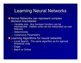
Outline Biological neural networks Artificial NN basics and training: – perceptrons – multi‐layer networks Combination with other ML techniques – NN and Reinforcement Learning • e.g. AlphaGo – NN and Evolutionary Computing 3
(Artificial) Neural Networks Supervised learning technique: error‐driven classification Output is weighted function of inputs Training updates the weights Used in games for e.g. – Select weapon – Select item to pick up – Steer a car on a circuit – Recognize characters – Recognize face – … 4
Biological Neural Nets Pigeons as art experts (Watanabe et al. 1995) – Experiment: • Pigeon in Skinner box • Present paintings of two different artists (e.g. Chagall / Van Gogh) • Reward for pecking when presented a particular artist (e.g. Van Gogh) 5
6
Results from experiment Pigeons were able to discriminate between Van Gogh and Chagall: with 95% accuracy, when presented with pictures they had been trained on still 85% successful for previously unseen paintings of the artists 7
Praise to neural nets Pigeons have acquired knowledge about art – Pigeons do not simply memorise the pictures – They can extract and recognise patterns (the ‘style’) – They generalise from the already seen to make predictions Pigeons have learned. Can one implement this using an artificial neural network? 8
Inspiration from biology If a pigeon can do it, how hard can it be? ANN’s are biologically inspired. ANN’s are not duplicates of brains (and don’t try to be)! 9
(Natural) Neurons Natural neurons: receive signals through synapses (~ inputs) If signals strong enough (~ above some threshold ), – the neuron is activated – and emits a signal though the axon . (~ output ) Artificial neuron (Node) Natural neuron 10
McCulloch & Pitts model (1943) “A logical calculus of the ideas immanent in nervous activity” Linear x 1 w 1 hard Combiner output delimiter x 2 w 2 y aka: - linear threshold gate w n x n - threshold logic unit • n binary inputs x i and 1 binary output y • n weights w i ϵ {‐1,1} � • Linear combiner: z = ∑ 𝑥 � 𝑦 � ��� • Hard delimiter: unit step function at threshold θ , i.e. 𝑧 � 1 if 𝑨 � 𝜄, 𝑧 � 0 if 𝑨 � 𝜄 11
Rosenblatt’s Perceptron (1958) x z y = g(z) x • enhanced version of McCulloch‐Pitts artificial neuron • n+ 1 real‐valued inputs : x 1 … x n and 1 bias b ; binary output y • weights w i with real‐valued values � • Linear combiner: z = ∑ 𝑥 � 𝑦 � � 𝑐 ��� • g(z) : (hard delimiter) unit step function at threshold 0, i.e. 𝑧 � 1 if 𝑨 � 0 , 𝑧 � 0 if 𝑨 � 0 12
Classification: feedforward The algorithm for computing outputs from inputs in perceptron neurons is the feedforward algorithm. 4 w=2 8 -4 0 w=4 -3 -12 0 weighted input: activation g(z) : 0 � z = � � ��� 0 13
Bias & threshold implementation Bias can be incorporated in three different ways, with same effect on output: ∑ ∑ b w 0 = 1 θ - b 1 b Alternatively: threshold θ can be incorporated in three different ways, with same effect on output… 14
Single layer perceptron Input Single layer of nodes: neurons: • Rosenblatt’s perceptron is building w 13 y 1 3 x 1 1 block of single‐layer perceptron w 14 w 23 • which is the simplest feedforward y 2 x 2 2 4 w 24 neural network • alternative hard‐limiting activation functions g(z) possible; e.g. sign function: 𝑧 � �1 if 𝑨 � 0 , 𝑧 � �1 if 𝑨 � 0 • can have multiple independent outputs y i • the adjustable weights can be trained using training data • the Perceptron learning rule adjusts the weights w 1 …w n such that the inputs x 1 …x n give rise to the (desired) output(s) 15
Perceptron learning: idea Idea: minimize error in the output per output: 𝑓 � 𝑒 � 𝑧 ( d =desired output) � If 𝑓 � 1 then z � ∑ 𝑥 � 𝑦 � should be increased such that it ��� exceeds the threshold � If 𝑓 � �1 then z � ∑ 𝑥 � 𝑦 � should be decreased such ��� that it falls below the threshold �� change 𝑥 � ← 𝑥 � +/‐ term proportional to gradient �� � � 𝑦 � Proportional change: learning rate 𝛽 > 0 NB in the book the learning rate is called Gain, with notation η 16
Perceptron learning Initialize weights and threshold (or bias) to random numbers; Choose a learning rate 0 � 𝛽 � 1 For each training input t =< x 1 ,…,x n >: 1 ‘epoch ’ calculate the output y(t) and error e(t)=d(t) - y(t) desired output Adjust all n weights using perceptron learning rule: 𝑥 � ← 𝑥 � � ∆𝑥 � where ∆𝑥 � � 𝛽 𝑦 � e(t) All Weights unchanged ? Weights for any t changed? Ready or other stopping rule… 17
Example: AND- learning (1) x 1 x 2 d x 2 0 0 0 1 0 1 0 1 0 0 1 1 1 x 1 0 1 d esired output of logical AND, given 2 binary inputs 18
Example AND (2) x 1 0 w=0.3 0 0 0 x 2 w=-0.1 0 0 e(t 1 ) = d(t) – 0 0.2 = 0 – 0 Init: choose weights w i and threshold θ randomly in [‐0.5,0.5]; set ; use step function : return 0 if < θ ; 1 if ≥ θ x 1 x 2 d(t) Alternative: use bias b= – θ t 1 0 0 0 with unit stepfunction t 2 0 1 0 t 3 1 0 0 Done with t 1 , for now… t 4 1 1 1 19
Example AND (3) x 1 0 w=0.3 0 -0.1 0 x 2 w=-0.1 1 -0.1 e(t 2 ) = 0-0 0.2 x 1 x 2 d(t) t 1 0 0 0 t 2 0 1 0 t 3 1 0 0 Done with t 2 , for now… t 4 1 1 1 20
Example AND (4) x 1 1 w=0.3 w=0.2 0.3 0.3 1 x 2 w=-0.1 0 0 e(t 3 ) = 0 - 1 0.2 � (t) x 1 x 2 d(t) � t 1 0 0 0 � t 2 0 1 0 t 3 1 0 0 � 1 1 1 t 4 w 1 0.2; done with t 3 , for now… 21
Example AND (5) x 1 w=0.2 1 w=0.3 0.2 0.1 0 x 2 w=0 w=-0.1 1 -0.1 e(t 4 ) = 1-0 0.2 x 1 x 2 d(t) � (t) � t 1 0 0 0 � t 2 0 1 0 .1 t 3 1 0 0 � t 4 1 1 1 w 1 0.3 and w 2 0; done with t 4 and first epoch… 22
Example (6) : 4 epoch’s later… x 1 w=0.1 x 2 w=0.1 0.2 algorithm has converged, i.e. the weights do not change any more. algorithm has correctly learned the AND function 23
AND example (7): results x 2 x 1 x 2 d y 0 0 0 0 1 0 1 0 0 1 0 0 0 1 1 1 1 x 1 0 1 Learned function/decision boundary: 0.1 𝑦 � � 0.1 𝑦 � � 0.2 linear classifier 𝑦 � � 2 � 𝑦 � Or : 24
Perceptron learning: properties All linear functions space without local optima Complete: yes, if – 𝛽 sufficiently small or initial weights sufficiently large – examples come from a linearly separable function! then perceptron learning converges to a solution. Optimal: no (weights serve to correctly separate ‘seen’ inputs; no guarantees for ‘unseen’ inputs close to the decision boundaries) 25
Limitation of perceptron: example x 2 XOR x 1 x 2 d 1 0 0 0 0 1 1 1 0 1 1 1 0 x 1 0 1 Cannot separate two output types with a single linear function XOR is not linearly separable. 26
Solving XOR using 2 single layer perceptrons x 1 x 1 ϴ =1 ϴ =1 x 1 1 1 ϴ =1 3 -1 1 1 1 y 3 -1 1 y 5 -1 4 4 y 2 2 1 -1 2 1 1 ϴ =1 x 2 x 2 ϴ =1 x 2 x 2 x 2 x 2 1 1 1 x 1 x 1 x 1 0 0 0 1 1 1 27
Types of decision regions 28
Multi-layer networks x 1 y 1 x 2 y 2 x 3 y 3 input hidden output nodes layer of neuron neurons layer • This type of network is also called a feed forward network • hidden layer captures nonlinearities • more than 1 hidden layer is possible, but often reducible to 1 hidden layer • introduced in 50s, but not studied until 80s 29
Multi-Layer Networks In MLNs outputs not based on simple weighted sum of inputs weights are shared dependent outputs Input signals x 1 y 1 x 2 y 2 x 3 y 3 Error signals errors must be distributed over hidden neurons continuous activation functions are used 30
Continuous activation functions As continuous activation function, we can use • a (piecewise) linear function (ReLU) • a sigmoid (smoothed version of step function) e.g. logistic sigmoid g(z) �� � z 31
Continuous artificial neurons Linear x 1 w 1 sigmoid Combiner output function x 2 w 2 y w n x n weighted input: activation ( logistic sigmoid ): z = 32
Example w=2 3 6 -2 0.119 w=4 -2 -8 weighted input: activation: z = 33
Error minimization in MLNs: idea Idea: minimize error in output through gradient descent Total error is sum of squared error, per output: 𝐹 � ∑ � � 𝑒 � 𝑧 � � ( d =desired output) � �� change 𝑥 � ← 𝑥 � � term proportional to gradient �� � 34
Recommend


More recommend
Explore More Topics
Stay informed with curated content and fresh updates.