Announcements Dont forget about Problem Set 4 Midterm 2 is getting - PowerPoint PPT Presentation

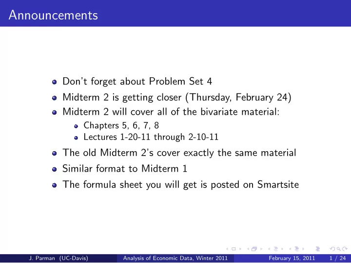
Announcements Don’t forget about Problem Set 4 Midterm 2 is getting closer (Thursday, February 24) Midterm 2 will cover all of the bivariate material: Chapters 5, 6, 7, 8 Lectures 1-20-11 through 2-10-11 The old Midterm 2’s cover exactly the same material Similar format to Midterm 1 The formula sheet you will get is posted on Smartsite J. Parman (UC-Davis) Analysis of Economic Data, Winter 2011 February 15, 2011 1 / 24

Multivariate Data annual salary, millions $ assists per game points per game J. Parman (UC-Davis) Analysis of Economic Data, Winter 2011 February 15, 2011 2 / 24

Multivariate Data: Overview We have seen how to analyze univariate data and bivariate data Now it is time to move on to working with more than two variables This is going to require a different set of techniques Most of what we do in economics uses more than two variables, even if the question of interest is the relationship between x and y Why? Because we’re never in a controlled environment, there are lots of things other than x and y moving around J. Parman (UC-Davis) Analysis of Economic Data, Winter 2011 February 15, 2011 3 / 24

Multivariate Data: Overview The general plan for studying multivariate data: Data description: graphical techniques Data description: regression Statistical inference: single slope (t-stats) Statistical inference: multiple slopes simultaneously (F-stats) J. Parman (UC-Davis) Analysis of Economic Data, Winter 2011 February 15, 2011 4 / 24

Graphing Multivariate Data With three variables, you can do a three-way scatter plot (or a surface) With three variables, you can also do a bubble chart (scatter plot with points of varying size) With additional variables, you have to start getting creative (3-D surface with color, animation to show a time dimension, bubble plot with different colors, etc.) An alternative is to produce a scatterplot for every pairing of variables (doesn’t really capture multivariate interactions) To Excel for a bubble plot example (nba-data.xlsx)... J. Parman (UC-Davis) Analysis of Economic Data, Winter 2011 February 15, 2011 5 / 24

Graphing Multivariate Data J. Parman (UC-Davis) Analysis of Economic Data, Winter 2011 February 15, 2011 6 / 24

Graphing Multivariate Data 5 4 missions per capita) 3 2 1 0 ‐ 1 1 4 4 5 5 6 6 7 7 8 8 9 9 10 10 11 11 ln(CO2 em ‐ 2 ‐ 3 ‐ 4 ‐ 5 ln(consumption per capita) Size of data points is proportional to GDP per capita. J. Parman (UC-Davis) Analysis of Economic Data, Winter 2011 February 15, 2011 7 / 24

Graphing Multivariate Data 45 45 45 45 40 40 40 40 35 35 35 City miles per gallon City miles per gallon City miles per gallon 30 30 30 25 25 25 Compact Compact Compact 20 20 20 Mid ‐ size Mid ‐ size Mid ‐ size 15 15 15 Large Large Large 10 10 10 5 5 0 0 0 0 1 1 2 2 3 3 4 4 5 5 6 6 7 7 8 8 Engine displacement (liters) Engine displacement (liters) J. Parman (UC-Davis) Analysis of Economic Data, Winter 2011 February 15, 2011 8 / 24

Graphing Multivariate Data From Natural Autoantibodies Reactive With Glycosaminoglycansin RA: Results, Gyorgy et al, Arthritis Research & Therapy. 2008;10(5) J. Parman (UC-Davis) Analysis of Economic Data, Winter 2011 February 15, 2011 9 / 24

Describing Multivariate Data with a Regression Graphs aren’t going to get us too far with multivariate data Instead, the most common approach is to use a multivariate regression This approach assumes that we have one dependent variable of interest ( y ) Now, we have several independent variables and need a little new notation J. Parman (UC-Davis) Analysis of Economic Data, Winter 2011 February 15, 2011 10 / 24

Multivariate Regression We now have K random variables: Y : dependent variable, outcome, left-hand-side (LHS) variable X 2 , ..., X K : covariates, explanatory variables, independent variables, right-hand-side (RHS) variables, regressors With these K variables, we also have K unknown population parameters ( K different β ’s) J. Parman (UC-Davis) Analysis of Economic Data, Winter 2011 February 15, 2011 11 / 24

Multivariate Regression Our model is now: Y = β 1 + β 2 X 2 + β 3 X 3 + ... + β K X K + ε We want to estimate a ’best-fit’ line: y i = b 1 + b 2 x 2 i + b 3 x 3 i + ... + b K x Ki ˆ y i : predicted value of Y for individual i ˆ x 2 i , ..., x Ki : values of X 2 , ..., X K for individual i b 1 : intercept b k : predicted ∆ Y for a one unit increase in X k holding all other X’s constant J. Parman (UC-Davis) Analysis of Economic Data, Winter 2011 February 15, 2011 12 / 24

Multivariate Regression As an illustration, let’s think about a wage regression Suppose we think wage ( w ) is a function of education ( edu ) and ( age ) so we estimate the following best fit line: w i = b 1 + b 2 edu i + b 3 age i ˆ ∆ w b 2 is telling us ∆ edu when age is held constant ∆ w b 3 is telling us ∆ age when education is held constant Note that these are not the same as the coefficients from doing two bivariate regressions (a bivariate regression doesn’t hold omitted variables constant) J. Parman (UC-Davis) Analysis of Economic Data, Winter 2011 February 15, 2011 13 / 24

Multivariate Regression J. Parman (UC-Davis) Analysis of Economic Data, Winter 2011 February 15, 2011 14 / 24

Multivariate Regression So how do we get this best fit line? Same way as before, minimize the distance of the y i values from the line Recall that we did this by minimizing the average squared deviation of each y i from the line (the residual): n min 1 � y i ) 2 ( y i − ˆ n i =1 The difference now is that the minimization is done by choosing the values of K different coefficients J. Parman (UC-Davis) Analysis of Economic Data, Winter 2011 February 15, 2011 15 / 24

Multivariate Regression n 1 � y i ) 2 min ( y i − ˆ n b 1 ,..., b K i =1 n 1 � ( y i − b 1 − b 2 x 2 i − ... − b K x Ki ) 2 min n b 1 ,..., b K i =1 To minimize this, we would take a derivative with respect to each b k and set it equal to zero This would give us K different equations to solve for K different unknowns The solution gives us a way to calculate each b k as a function of our data J. Parman (UC-Davis) Analysis of Economic Data, Winter 2011 February 15, 2011 16 / 24

Multivariate Regression The coefficients aren’t hard to calculate if you know a little matrix algebra We’ll just use Excel’s regression option to calculate them In Excel, choose Regression from the Data Analysis menu When you choose your x data, select all of the columns containing your independent variables (these columns need to be side by side) The regression output will contain coefficients, standard errors, etc. for all of the variables To Excel and the NBA data... J. Parman (UC-Davis) Analysis of Economic Data, Winter 2011 February 15, 2011 17 / 24

Multivariate Regression: Interpreting the Results SUMMARY OUTPUT: ln(salary in millions) as dependent variable Regression Statistics Regression Statistics Multiple R 0.63293872 R Square 0.40061142 Adjusted R Square 0.39612162 Standard Error 0.68450419 Observations 270 Coefficients Standard Error t Stat P ‐ value Intercept ‐ 0.9728428 0.087267003 ‐ 11.1479 5.98E ‐ 24 points 0.07408318 0.008560474 8.654098 4.76E ‐ 16 rebounds 0.06056555 0.017484676 3.463922 0.00062 J. Parman (UC-Davis) Analysis of Economic Data, Winter 2011 February 15, 2011 18 / 24

Multivariate Regression: Goodness of Fit We can use the same methods as before to measure how good the fit of the regression line is: The standard error of the regression The R 2 We also have another measure called the adjusted R 2 All of these measures are reported in Excel’s regression output J. Parman (UC-Davis) Analysis of Economic Data, Winter 2011 February 15, 2011 19 / 24

Multivariate Regression: Goodness of Fit The standard error of the regression: � n � 1 � � y i ) 2 s e = ( y i − ˆ � n − K i =1 This measures the average squared deviation of each y i from its predicted value It will be smaller the better our fit is but its magnitude depends on the units in which we measure y J. Parman (UC-Davis) Analysis of Economic Data, Winter 2011 February 15, 2011 20 / 24

Multivariate Regression: Goodness of Fit The R 2 : R 2 = 1 − ESS TSS n � y i ) 2 ESS = ( y i − ˆ i =1 n � y ) 2 TSS = ( y i − ¯ i =1 R 2 will be between 0 and 1, the closer it is to 1 the better the fit is J. Parman (UC-Davis) Analysis of Economic Data, Winter 2011 February 15, 2011 21 / 24

Multivariate Regression: Goodness of Fit The problem with R 2 is that it will automatically increase (or at least stay the same) whenever we add more regressors We would like a measure that takes into account the number of regressors we use For example, we might prefer a line that gives us an R 2 of .8 with only three regressors to a line that gives us an R 2 of .81 but uses thirty regressors The adjusted R 2 is a variation on R 2 that penalizes models that use may variables J. Parman (UC-Davis) Analysis of Economic Data, Winter 2011 February 15, 2011 22 / 24