Announcements CS 4100: Artificial Intelligence Markov Decision - PDF document

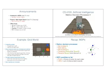
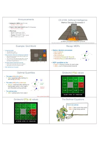
Announcements CS 4100: Artificial Intelligence Markov Decision Processes • Homework k 3: Game Trees s (lead TA: Zhaoqing) • Due Tue 1 Oct at 11:59pm (deadline extended) • Homework k 4: MDPs s (lead TA: Iris) • Due Mon 7 Oct at 11:59pm • Pr Project 2 t 2: Mu Multi-Ag Agent Search (lead TA: Zhaoqing) • Due Thu 10 Oct at 11:59pm • Offi Office H Hours • Iris: s: Mon 10.00am-noon, RI 237 • JW JW: Tue 1.40pm-2.40pm, DG 111 • Zh Jan-Willem van de Meent Zhaoqi qing: : Thu 9.00am-11.00am, HS 202 • El Eli: Fri 10.00am-noon, RY 207 Northeastern University [These slides were created by Dan Klein and Pieter Abbeel for CS188 Intro to AI at UC Berkeley. All CS188 materials are available at http://ai.berkeley.edu.] Non-Deterministic Search Example: Grid World A maze-like A ke problem • • The agent lives in a grid Walls block the agent’s path • • No Nois isy movement: act actions s do o not ot al always ays go as as plan anned ed • 80% of the time, the action North takes the agent North (if there is no wall there) • 10% of the time, North takes the agent West; 10% East If there is a wall in the direction the agent would have • been taken, the agent stays put • The The age gent nt receives s rewards s each h time st step Small “living” reward each step (can be negative) • • Big rewards come at the end (good or bad) Go Goal: l: maxim imiz ize sum of rewa wards • Grid World Actions Markov Decision Processes Determ De rmin inis istic ic Grid rid World rld St Stochastic Grid World • An MDP is s defined by • A se s Î S set of st states s • A se a Î A set of actions s a • A transi sition function T(s, s, a, s’) ’) • Probability that a a from s leads to s’ s’ , i.e., P(s P(s’| s, s, a) • Also called the model or the dynamics • A re reward rd function R(s, s, a, s’) ’) • Sometimes just R(s) s) or R( R(s’) ’) • A st start st state • Maybe a terminal st state • MDPs s are non-determinist stic se search problems • One way to solve them is with exp xpectimax search • We’ll have a new tool soon [Demo – gridworld manual intro (L8D1)] What is Markov about MDPs? Policies • “Marko • kov” v” generally means that given the current st state , In determinist stic si single-agent se search problems , we wanted an optimal pl plan , or sequence of the future and the past st are independent actions, from start to a goal • For Marko kov v decisi sion processe sses , “Markov” means y p *: • For MD MDPs , we want an optimal policy *: S → A action outcomes s depend only on the current st state A policy p gives an acti • action on for each st state • An optimal policy is one that maxi ximize zes s exp xpected utility y • An exp xplicit policy defines a reflex x agent Andrey Markov (1856-1922) Optimal policy when R(s, a, s’) = -0.03 • xpectimax didn’t compute entire policies Exp for all non-terminals s • It computed the action for a single state only • This is just like search, where the successor function could only depend on the current state (not the history)

Optimal Policies Example: Racing R(s) = -0.01 R(s) = -0.03 R(s) = -0.4 R(s) = -2.0 Example: Racing Racing Search Tree • A robot car wants to travel far, quickly • Three states: Cool, Warm, Overheated Two actions: Slow , Fast • 0.5 +1 • Going faster gets double reward 1.0 Fast Slow -10 +1 0.5 Warm Slow Fast 0.5 +2 Cool 0.5 Overheated +1 1.0 +2 MDP Search Trees Utilities of Sequences • Each MDP st state projects s an exp xpectimax-like ke se search tree s is a state s a (s, a) (s a) is a s, a q-st state ( s, s,a,s ’ ) is called a tr transitio ition T(s, T( s,a,s ’ ) ) = P(s P(s ’ |s, s,a) s,a,s ’ R( R(s, s,a,s ’ ) s ’ Utilities of Sequences Discounting • It’s reasonable to maxi ximize ze the su sum of rewards • What preferences should an agent have over reward sequences? • It’s also reasonable to pr prefer rewards s now to rewards s later • One so [1, 2, 2] or [2, 3, 4] solution: values of rewards decay y exp xponentially • More or less? [0, 0, 1] or [1, 0, 0] • Now or later? Worth Now Worth Next Step Worth In Two Steps

<latexit sha1_base64="AGurigOo2orwZWQwqUQeS/5KGPs=">AGXnicfZTNbtQwEIDd0m5LoLSFCxKXFXvhsFqS3artBakquBYqv5J9VI5zmzWav7WdtpuLT8dT8GNa6/wAji7ATZxhCNFo5lvPGPePwsYkK67vel5Scrq6219afOs+cbLza3tl+eizTnFM5oGqX80icCIpbAmWQygsuMA4n9C78m4+F/eIWuGBpciqnGQxjEiZsxCiRnW9NcQhiWPydDGNEhl23PbH9pz3R+NgyeTnAQO5iwcS8J5evdXNQeNh5hwqbz3nquNzGKYtN3eoH+91XF7my1bcErhc4Bmq/j6+2VRxykNI8hkTQiQlx5biaHinDJaATawbmAjNAbEsKVERMSgxiq2T3odsV6g3VKE0kJLTipkgsYiLHlrKARVLxyYw8GrYUjlUxS4BCBYmVS8/1o6DAxiZmswyU4Ef5aDVyadDrdzu7qDr9fd0DeEQlIS373bNVwdCDpCUyP5O19vdt5ks51kE/yC3wIpsOCRwR1NTrSRQ+BaovjL3gyEROYfiIAr7sep4WmsLnqPGZ2Z38KLxXiuFKwniW3Wv69h0ASsOaqCpBT07fVgYZMmDMsxSNKQvWymSd7A5hab2xC3IF7PEBpjQiZYlCbWeUYL9KxPRnbQaIEpa1xsGZmHhBrx2zcjGdjZrEntcqc6KJdFgnCw5iYOuM0A05kyotHd8fkOGIxk0KVdm17seT/XsZeD3akq01Z/H1fHWmLpH40a8zq3dkdSnlQ5YpTNmAhr2LzwjWAWQ0sL3hGVuZARCTci2lcnQ7gZzxNR9oxw9Grj0JbO/3vEGv/2Wnc3BYjsl19Aa9Re+Qh/bQAfqMjtEZougbekQ/0a/VH61Wa6O1OUeXl0qfV6iyWq9/A/fVUqw=</latexit> Discounting Stationary Preferences • Theorem: Theorem: if we assume st stationary y preferences • How to disc scount? • Each time we descend a level, we multiply in the discount once • Why y disc scount? • Sooner rewards probably do have higher utility than later rewards • Also helps our algorithms converge • Then: Then: there are only two ways to define ut utilities es • Exa xample: disc scount of 0. 0.5 • Additive ve utility: y: • U( U([1,2 ,2,3 ,3]) = = 1 1*1 + + 0 0.5 .5*2 + + 0 0.2 .25*3 • U( U([1,2 ,2,3 ,3]) < < U( U([3,2 ,2,1 ,1]) • Disc scounted utility: y: Exercise: Discounting Exercise: Discounting • Give • Give ven: ven: • Actions: • Actions: s: East st , West st , and Exi xit (only available in exit states a , e ) s: East st , West st , and Exi xit (only available in exit states a , e ) • Transi • Transi sitions: s: determinist stic sitions: s: determinist stic • Quiz z 1: For g = • Quiz z 1: For g = = 1 , what is the optimal policy? = 1 , what is the optimal policy? z 2: For g = z 2: For g = • Quiz • Quiz = 0.1 , what is the optimal policy? = 0.1 , what is the optimal policy? z 3: For which g are West z 3: For which g are West • Quiz • Quiz st and East st equally good when in state d ? st and East st equally good when in state d ? ∆ γ 3 · 10 = γ · 1 γ = 1 / 10 ' 0.32 ! Infinite Utilities?! Recap: Defining MDPs • Pr Probl blem: What if the game lasts forever? Do we get infinite rewards? • Marko kov v decisi sion processe sses: s: s • Set of st states S • Solutions: s: a • Start st state s 0 • Finite horizo zon: (similar to depth-limited search) • Se s, a Set of actions A • Terminate episodes after a fixed T steps (e.g. life) • Transi sitions P( P(s’ s’|s, s,a) (or T( T(s, s,a,s’) ’) ) stationary policies ( p depends on time left) • Gives nonst s,a,s ’ s,a,s’) (and discount g ) • Re Rewards R( R(s, < g < • Disc scounting: use 0 0 < < 1 s ’ • MDP quantities s so so far: • Po • Smaller g means smaller “horizo Policy = Choice of action for each state zon” – shorter term focus • Ut Utilit ility = sum of (discounted) rewards • Abso sorbing st state: guarantee that for every policy, a terminal state will eventually be reached (like “overheated” for racing) Solving MDPs Optimal Quantities Th The value (uti utility ty) ) of f a st state s • V * (s (s) = expected utility starting in s s • and acting opt optima mally s is a s state a • The value (uti Th utility ty) ) of f a q-st state (s, s,a) (s, a) is a s, a q-state • Q * (s, s,a) = expected utility starting out having taken action a from state s s s,a,s’ (s,a,s’) is a and (thereafter) acting optimally transition s’ The opt Th optima mal pol policy • p * (s (s) ) = optimal action from state s • [Demo – gridworld values (L8D4)]

Gridworld V values Gridworld Q Q values Noise = 0.2 Noise = 0.2 Discount = 0.9 Discount = 0.9 Living reward = 0 Living reward = 0 Values of States Racing Search Tree • Fund Fundament amental al op operat eration: on: compute the exp xpectimax va value of a state • Expected utility under optimal action s • Average sum of (discounted) rewards a • This is just what expectimax computed! s, a • Recursi sive ve definition of va value (Bellman Equations) s): s,a,s ’ s ’ Racing Search Tree Racing Search Tree • We’re doing way y too much work k with exp xpectimax! • Pr Probl blem: : States are repeated • Id Idea: Only compute needed quantities once • Pr Probl blem: Tree goes on forever • Id Idea: Do a depth-limited computation, but with increasing depths until change is small • No te: deep parts of the tree Note eventually don’t matter if γ < < 1 Time-Limited Values k=0 • Key y idea: time-limited values • De s) to be the optimal value of s if the Defin ine V k (s) game ends in k more time steps • Equivalently, it’s what a de dept pth-k exp xpectimax would give from s Noise = 0.2 Discount = 0.9 [Demo – time-limited values (L8D6)] Living reward = 0