and ( ) ( ) , F , P , , P . 1 Combining both models, - PDF document
HEDGING METHODOLOGIES IN EQUITY-LINKED LIFE INSURANCE Alexander Melnikov University of Alberta, Edmonton e-mail: melnikov@ualberta.ca 1. Formulation of the Problem and Introductory Remarks. The contracts we are going to study have two types of
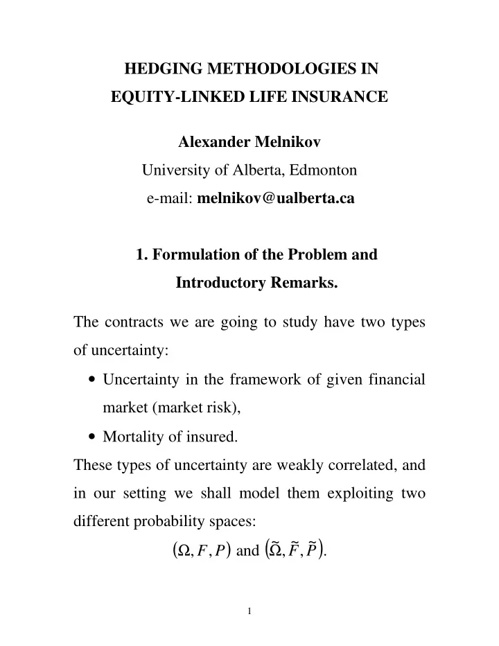
HEDGING METHODOLOGIES IN EQUITY-LINKED LIFE INSURANCE Alexander Melnikov University of Alberta, Edmonton e-mail: melnikov@ualberta.ca 1. Formulation of the Problem and Introductory Remarks. The contracts we are going to study have two types of uncertainty: • Uncertainty in the framework of given financial market (market risk), • Mortality of insured. These types of uncertainty are weakly correlated, and in our setting we shall model them exploiting two different probability spaces: ~ F ~ ~ and ( ) ( ) Ω Ω , F , P , , P . 1
Combining both models, we get the product space ~ ~ ~ ( ) Ω × Ω × × , F F , P P . Financial Market is represented by a pair of assets, non-risky B and risky S , that are identified by their prices ( B and ( ) ) S as stochastic processes on t t ( ) Ω , F , . P = Assuming for simplicity B 1 , we describe a t filtration ( { } ) = = σ F F S 0 ..., , S t t ≥ t 0 as the available information about prices at time t . To give a full description of the market, we should introduce a variety of admissible operations with the basic assets, B and S . Define a 2-dimensional stochastic process ( ) π = β γ , (usually predictable) adapted to F , as a t t t portfolio , or a strategy with the value (capital) π = β + γ X B S . t t t t t 2
π If X follows the equation t π = β + γ dX dB dS , t t t t t then we call π self-financing . Only portfolios with non-negative capital are admissible in the framework of the market. Any financial contract is identified with its potential liability (payoff) H , exercised at the end of a contract period [ ] 0 , T . In fact, H is a F -measurable random T variable. Any such nonnegative random variable H is called a contingent claim . In financial economics, a contingent claim is called a derivative security of the European type. Remark: A larger class of derivative securities, the American type, is not considered here. The main problem is to find the current price of a given contingent claim during a contract period [ ] 0 , T in order to manage the risk in the framework of the contract. 3
An appropriate solution is found by hedging the contingent claims: to construct an admissible strategy π so that * π * X is close enough to H T in some probabilistic sense. Hedging gives us a possibility to determine the t ≤ current price C at time T as the current capital t π * = π . C X of the hedging portfolio * t t In particular, π * = C X 0 represents the initial price of the claim. 4
Types of hedging 1. Perfect hedging: { } 1 π * ≥ H = P X . T 2. Mean-variance hedging: ( ) 2 π * T − E X H is minimal. 3. Efficient hedging: { ( ) } π + * − E l H X is minimal, T where l is a loss function. In particular, for quantile hedging, we have ( ) ) ( ) = l x I x and ( ∞ 0 , { } π * ≥ P X H is maximal. T 5
How to calculate the price C ? To answer this question, we use the martingale characterization of arbitrage and completeness of a financial market (in terms of existence and uniqueness of risk-neutral or martingale measures) given by the first and the second fundamental theorems in financial mathematics. So, we reduce the method of risk-neutral valuation of the contingent claim H to finding the price C as t = C , E * ( H | F ) t t where E is an expectation w.r. to a single * martingale measure P (complete market) or * = C sup E * ( H | F ) t t P * (incomplete market). 6
Life insurance contracts based on risky assets The source of randomness in financial contracts is the evolution of stock prices. The source of randomness in life insurance is the mortality of clients. Denote ( ) T x a random variable representing the future ( ) lifetime of a client of age x . T x is given on ~ F ~ ~ ( ) Ω , , . P An insurance company can issue a mixed contract for the period [ ] 0 , T , where the payoff function is a and ( ) function of stock prices S , ..., S T x . 0 T This type of contract is called equity-linked life insurance contract . We will consider only pure endowment contracts with the following structure of payoffs: = ⋅ . H ( T ( x )) H I { ( ) } T x > T 7
Remarks: (1) Traditional life insurance deals with = = the deterministic payoff H K const . The price of K ⋅ the contract is equal to T p , where x = ~ { ( ) } > p x P T x T is a survival probability of the T insured of age x . (2) Pure endowment with a fixed guarantee : { } = ⋅ H ( T ( x )) max S , K I , { } > T T ( x ) T where S is a risky asset, K is a guarantee. (3) Pure endowment with a flexible guarantee : { } 1 , 2 = ⋅ H ( T ( x )) max S S I , { } T T T ( x ) > T 1 2 where S is the risky asset, S is the flexible (may be T T also a risky asset) guarantee. Assume that S in (2) follows geometric Brownian Motion (Black-Scholes model): � � 2 � � σ � � � � = µ − + σ ≤ S S exp t W , t T , t 0 � � t � 2 � where W is a Wiener process, µ is a rate of return on stock S , and σ is the volatility. 8
A Brief History We note the papers by Brennan and Schwartz (1976,1979), Boyle and Schwartz (1977), which recognized a close connection of equity-linked life insurance with the option pricing theory (Black, Scholes, and Merton (1973)). They found that the payoff from equity-linked life insurance contract at expiration is identical to the payoff from a European call option plus some guaranteed amount. Hence, the appearance of Black-Scholes formula in such pricing is quite natural in the construction of the initial price and the value of the portfolio: [ ] ( ) ( ) = Φ + Φ − U p S d K d + − T x T x 0 [ ( ) ( ) ] , = + Φ − Φ − p K p S d K d T x T x 0 + − 2 σ S 2 0 ± ln T y − 1 x K 2 2 ( ) � = Φ = e dy d , x . ± σ π T 2 − ∞ 9
Further developments: Delbaen (1986), Bacinello and Ortu (1993), Aase and Persson (1994). The important step was done by Moeller (1998, 2001, 2002) who applied the mean-variance hedging technique. He obtained the following result: [ ( ) ( ) ] = ⋅ Φ + Φ − U ( T , l ) l p S d K d + − x x T x 0 * ( ) ( ) ′ γ = − and l N p F t , S t x t − T − t x + t x t give the initial price and optimal (in the mean- variance sense) hedging strategy for the contract of pure endowment with a guarantee K for a group of clients of age x , where x l is the size of the group of the insured with the remaining life times ( ) ( ) T x ,..., T x , 1 l x l ~ x � ( ) = = + > − , ( ) . N I p P T x t T t { ( ) } t T x ≤ t T − t x + t i i i = 1 ( ) F , t x satisfies the Black-Scholes fundamental equation ( ) = r 0 10
1 2 2 ( ) ( ) ′ ′ ′ + σ = F t , x x F t , x 0 t xx 2 with the boundary condition ( ) { } = F T , x max x , K . Remark: Our main focus is on calculating the premium T U for a single contract. Since for a group x of size x l we get = ⋅ U ( T , l ) l U . x x T x t ≤ Also, for every fixed T we can repeat the logical steps for the interval [ T t , ] and find the corresponding premiums as a product − ⋅ ( l N ) U . − + x t T t x t 11
2.Conditioned Contingent Claims in a semimartingale setting. Assume that the risky asset S is a semimartingale on ( ) = Ω S ( S t F , ) , F , F , P . t t ≤ T ( ) π = β γ A self-financing admissible strategy , t π π � = + γ ≥ has a capital X X dS 0 . t 0 u u 0 M ( S , P ) is a set of martingale measures of this * = market. Firstly, we assume that M ( S , P ) { P } . Consider a nonnegative contingent claim H which is * < ∞ F -measurable random variable with E H . t According to the risk-neutral valuation methodology, t * H � = = + γ ≥ C ( ) ( | ) C ( ) 0 , H E H F H dS t t 0 u u 0 * = C ( H ) E H , 0 ( ) H H H π = β γ , is a replicating portfolio (perfect hedge). 12
Consider a nonnegative random variable τ defined ~ F ~ ~ on another probability space ( ) Ω , , P and determine a conditioned contingent claim τ ) = ⋅ H ( H I { } τ > T ~ ~ ~ on the product space ( ) Ω × Ω × × , F F , P P . ( τ To price H ) we consider the value ~ ~ * * τ = × τ = ⋅ C ( ) E E ( H ( )) E H E I { } τ > T = ⋅ < C ( H ) p ( T ) C ( H ) 0 0 ( τ as a bound for the initial price of H ) and define the set of successful hedging π π π π = ω ≥ A ( X , ) { : X ( X ) H } . 0 T 0 H π = π π = If then ( ( C ( ), )) 1 . We should P A H 0 consider a restricted set of strategies with the initial π ≤ = ⋅ capital X X C ( H ) p ( T ) . Thus, we cannot 0 0 0 provide the above equality. 13
Recommend
More recommend
Explore More Topics
Stay informed with curated content and fresh updates.















![CS171 Visualization Alexander Lex alex@seas.harvard.edu Graphs [xkcd] This Week Reading: VAD,](https://c.sambuz.com/709269/cs171-visualization-s.webp)
