Analyzing Marketing Data with an R- marketing actions, c.f. based - PowerPoint PPT Presentation
Marketing Problems Marketing is an applied field that seeks to optimize firm behavior with respect to a set of Analyzing Marketing Data with an R- marketing actions, c.f. based Bayesian Approach set prices optimally for a large number of
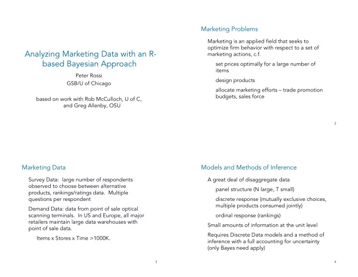
Marketing Problems Marketing is an applied field that seeks to optimize firm behavior with respect to a set of Analyzing Marketing Data with an R- marketing actions, c.f. based Bayesian Approach set prices optimally for a large number of items Peter Rossi design products GSB/U of Chicago allocate marketing efforts – trade promotion budgets, sales force based on work with Rob McCulloch, U of C, and Greg Allenby, OSU 2 Marketing Data Models and Methods of Inference Survey Data: large number of respondents A great deal of disaggregate data observed to choose between alternative panel structure (N large, T small) products, rankings/ratings data. Multiple questions per respondent discrete response (mutually exclusive choices, multiple products consumed jointly) Demand Data: data from point of sale optical scanning terminals. In US and Europe, all major ordinal response (rankings) retailers maintain large data warehouses with Small amounts of information at the unit level point of sale data. Requires Discrete Data models and a method of Items x Stores x Time >1000K. inference with a full accounting for uncertainty (only Bayes need apply) 3 4
Hierarchical Models A Graphical Review of Hierarchical Models A multi-level Model comprised of a set of θ τ y X conditional distributions: 1 1 1 � � “unit-level” model – distribution of response τ h θ τ given marketing variables y X i i i first stage prior – specifies distribution of � � response parameters over units θ τ y X m m m second stage prior – prior on parameters of first stage prior Second Stage Prior: First Stage Prior: “Unit-Level” Modular both conceptually and from a Adaptive Shrinkage Random Coef Likelihoods or Mixing Distribution computational point of view. 5 6 Hierarchical Models and Bayesian Inference Implementation in R ( bayesm ) Model to a Bayesian (Prior and Likelihood): Data Structures (all lists) rxxxYyyZzz(Prior, Data, Mcmc) ) ( ) ( ) ∏ ( ∏ θ τ τ × θ p p h p y X , i i i i Prior: list of hyperparms (defaults) i i Object of Interest for Inference (Posterior): Data: list of lists for panel data ( ) e.g. Data=list(regdata,Z) θ θ τ p , … , , y , … , y 1 m 1 m regdata[[i]]=list(y,X) Computational Method: Mcmc: Mcmc tuning parms MCMC (indirect simulation from joint e.g. R (# draws), thining parm, posterior) Metropolis scaling (with def) 7 8
Implementation in R ( bayesm ) Coding Output: “Chambers” Philosophy – code in R, profile and rewrite only where necessary. Resulted in ~5000 draws of model parameters: lines of R code and 500 of C list of lists (e.g. normal components) As amateur R coders, we use only a tiny subset 3 dim array (unit x coef x draw) of R language. Code is numerically efficient but does not use many features such as classes User Decisions: Moving toward more use of .Call to maximize “burn-in” / convergence of the chain use of R functions. run it longer! This maximizes readability of code. Numerical Efficiency ( numEff ) We hope others will extend and modify. how to summarize the joint distribution? 9 10 Hierarchical Models considered in bayesm Hierarchical Linear Model- rhierLinearModel Normal Prior rhierLinearModel Consider m regressions: Mixture of Normals rhierLinearMixed ( ) = β + ε ε σ 2 = MNL with mixture of Normals y X ∼ iidN 0, I i 1 , … , m rhierMnlRwMixed i i i i i i n i MNL with Dirichlet Process Prior rhierMnlRwDP ( ) β = β + Binary logit with Normal prior v v ∼ iidN 0, V rhierBinLogit β i i i Neg Bin with Normal Prior rhierNegBinRw Priors : Ordinal Probit with Scale Usage ( ) rscaleUsage ( ) β β − 1 υ υ ∼ N , A ; V ∼ IW , I Mixture of Normals density est β β rnmixGibbs DP Prior density est rDPGibbs Tie together via Prior 11 12
Adaptive Shrinkage An Example – Key Account Data y= log of sales of a “sliced cheese” product at a Δ ,V With fixed values of , we have m independent β “key” account – market retailer combination Bayes regressions with informative priors. X: log(price) In the hierarchical setting, we “learn” about the { } β i location and spread of the . display (dummy if on display in the store) weekly data on 88 accounts. Average account has 65 weeks of data. The extent of shrinkage, for any one unit, depends on dispersion of betas across units and the amount See data(cheese) of information available for that unit. 13 14 Intercept 13 Shrinkage 12 post mean 11 An Example – Key Account Data 10 9 Prior on is key. V β 8 8 9 10 11 12 13 ( ) Failure of Least υ υ V ~ IW , I ls coef β 2.0 Squares Display some 1.5 1.5 υ = + post mean blue : k 3 accounts 0.5 post mean 1.0 have no υ = + green : k .5 n -0.5 displays! υ = + yellow : k 2 n -0.5 0.0 0.5 1.0 1.5 2.0 0.5 some ls coef accounts LnPrice 0.0 Greatest have absurd -1.0 Shrinkage for post mean coefs -2.0 -0.5 Display, least for -3.0 0 5 10 15 20 25 -4.0 intercepts ls coef -4.0 -3.5 -3.0 -2.5 -2.0 -1.5 -1.0 -0.5 15 16 ls coef
Heterogeneous logit model Random effects with regressors ( ) β = Δ + ' z v v iidN 0, V ∼ Assume T h observations per respondent β h h i h or β exp[ x ' ] = ∑ = Pr( y i ) it h = Δ + B Z U jth β exp[ x ' ] jt h Priors : The posterior: j ( ) ( ) ( ) δ = Δ δ − υ υ 1 vec ∼ N , A ; V ∼ IW , I β β ⎛ ⎞ T H ∏ ∏ h ( ) ( ) ( ) β β ∝ β β τ τ p ({ }, , V | Data ) p y | X , p | p ⎜ ⎟ h β iht ht h h ⎝ ⎠ Δ is a matrix of regression coefficients related h = 1 t = 1 covariates (Z) to mean of random-effects distribution. z h are covariates for respondent h prior logit normal model heterogeneity 17 18 data(bank) data(bank) Not all possible combinations of attributes were Pairs of proto-type credit cards were offered to offered to each respondent. Logit structure respondents. The respondents were asked to (independence of irrelevant alternatives makes this choose between cards as defined by “attributes.” possible). Each respondent made between 13 and 17 14,799 comparisons made by 946 respondents. paired comparisons. ' β exp[ x ] Sample Attributes (14 in all): = Pr( card 1 chosen ) h i , ,1 h β + β exp[ x ' ] exp[ x ' ] Interest rate, annual fee, grace period, out-of- h i , ,1 h h i , ,2 h − β exp[( x x )' ] state or in-state bank, … = h i , ,1 h i , ,2 h differences in + − β 1 exp[( x x )' ] attributes is all that h i , ,1 h i , ,2 h matters 19 20
Sample demographics (Z) Sample observations respondent 1 choose first card on first pair. Card chosen id id age ag income in come gend gender er had attribute 1 on. Card not chosen had attribute 4 on. 1 60 20 1 2 40 40 1 3 75 30 0 4 40 40 0 6 30 30 0 choic choic 7 30 60 0 id id e d1 d1 d2 d2 d3 d3 d4 d4 d5 d5 d6 d6 d7 d7 d8 d8 d9 d9 d10 d10 d11 d11 d12 d12 d13 d13 d14 d14 8 50 50 1 1 1 1 0 0 -1 0 0 0 0 0 0 0 0 0 0 9 50 100 0 1 1 1 0 0 1 -1 0 0 0 0 0 0 0 0 0 10 50 50 0 1 1 1 0 0 0 1 -1 0 0 0 0 0 0 0 0 11 40 40 0 1 1 0 0 0 0 0 0 1 0 -1 0 0 0 0 0 12 30 30 0 1 1 0 0 0 0 0 0 1 0 1 -1 0 0 0 0 13 60 70 0 1 1 0 0 0 -1 0 0 0 0 0 0 1 -1 0 0 14 75 50 0 1 1 0 0 0 0 0 0 0 0 -1 0 0 0 -1 0 1 0 0 0 0 0 0 0 0 0 1 0 0 0 -1 0 2 1 1 0 0 -1 0 0 0 0 0 0 0 0 0 0 2 1 1 0 0 1 -1 0 0 0 0 0 0 0 0 0 21 22 rhierBinLogit Running rhierBinLogit (continued) z=read.table("bank.dat",header=TRUE) d=read.table("bank demo.dat",header=TRUE) Data=list(Dat=Dat,Demo=d) # center demo data so that mean of random-effects # distribution can be interpretted as the average respondents nxvar=14 d[,1]=rep(1,nrow(d)) ndvar=4 d[,2]=d[,2]-mean(d[,2]) nu=nxvar+5 d[,3]=d[,3]-mean(d[,3]) Prior=list(nu=nu,V0=nu*diag(rep(1,nxvar)), d[,4]=d[,4]-mean(d[,4]) deltabar=matrix(rep(0,nxvar*ndvar), hh=levels(factor(z$id)) ncol=nxvar), nhh=length(hh) Adelta=.01*diag(rep(1,ndvar))) Dat=NULL Mcmc=list(R=20000,sbeta=0.2,keep=20) for (i in 1:nhh) { out=rhierBinLogit(Prior=Prior,Data=Data,Mcmc=Mcmc) y=z[z[,1]==hh[i],2] nobs=length(y) X=as.matrix(z[z[,1]==hh[i],c(3:16)]) Dat[[i]]=list(y=y,X=X) } 23 24
Recommend
More recommend
Explore More Topics
Stay informed with curated content and fresh updates.

