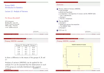
Analysis of variance April 16, 2009 Contents Comparison of several - PowerPoint PPT Presentation

Analysis of variance April 16, 2009

Contents • Comparison of several groups • One-way ANOVA • Two-way ANOVA – Interaction • Model checking Acknowledgement for use of presentation • Julie Lyng Forman, Dept. of Biostatistics (2008), • Lene Theil Skovgaard, Dept. of Biostatistics (2007, 2006)

Marc Andersen StatGroup ApS e-mail: mja@statgroup.dk http://staff.pubhealth.ku.dk/~pd/V+R/html/

ANOVA, April 2009 1 Comparison of 2 or more groups number different same of groups individuals individual 2 unpaired paired t-test t-test ≥ 2 one way two way analysis of variance analysis of variance One-way analysis of variance: • Do the distributions differ between the groups? • Do the levels differ between the groups?

ANOVA, April 2009 2 Example: 22 bypass-patients, 3 different kinds of ventilation during anaesthesia, randomized Group I 50% N 2 O, 50% O 2 for 24 hours Group II 50% N 2 O, 50% O 2 during operation Group III 30–50% O 2 (no N 2 O) for 24 hours Gr.I Gr.II Gr.III 8 9 5 n Mean 316.6 256.4 278.0 SD 58.7 37.1 33.8

ANOVA, April 2009 3

ANOVA, April 2009 4 One-way ANOVA • one-way : because we only have one critera for classification of the observations, here ventilation method • ANalysis Of VAriance : because we compare the variance between groups with the variance within groups

ANOVA, April 2009 5 Model: Y ij = µ i + ε ij j’th observation individual in group no. i deviation mean of group no. i Observations are assumed be independent and to follow a normal distribution (within each group) with the same variance . ε ij ∼ N (0 , σ 2 ) or equivalently Y ij ∼ N ( µ i , σ 2 ) Model assumptions must be checked!

ANOVA, April 2009 6 Hypothesis testing Usual approach • Null hypothesis: group means are equal, H 0 : µ i = µ • Alternative hypothesis: group means are not equal • We show the means are not equal by rejecting the null hypothesis of equality (ref DGA, 8.5 Hypothesis Testing)

ANOVA, April 2009 7 ANOVA math: Sums of squares Decomposition of ’deviation from grand mean’: y ij − ¯ y · = ( y ij − ¯ y i ) + (¯ y i − ¯ y · ) y ij j ’th observation in i ’th group y i ¯ average in i ’th group y . ¯ total average Decomposition of variation (sums of squares): � � � y · ) 2 y i ) 2 y · ) 2 ( y ij − ¯ = ( y ij − ¯ + (¯ y i − ¯ i,j i,j i,j � �� � � �� � � �� � total variation within groups between groups

ANOVA, April 2009 8 Decomposition of variation : total = between + within SS total = SS between + SS within ( n − 1) = ( k − 1) + ( n − k ) F-test statistic: F = MS between = SS between / ( k − 1) MS within SS within / ( N − k ) Reject the null hypothesis if F is large, i.e. if the variation between groups is too large compared to the variation within groups .

ANOVA, April 2009 9 Usually the analysis is summarized in an Analysis of variance table Variation df SS MS F P Between k − 1 SS b SS b / df b MS b / MS w P ( F (df b , df w ) > F obs ) Within n − k SS w SS w / df w Total n − 1 SS tot

ANOVA, April 2009 10 Analysis of variance table - Anaestesia example df SS MS F P Between 2 15515.88 7757.9 3.71 0.04 Within 19 39716.09 2090.3 Total 21 55231.97 F = 3 . 71 ∼ F (2 , 19) ⇒ P = 0 . 04 Weak evidence of non-equality of the three means

ANOVA, April 2009 11 Analysis of variance in SAS To define the anaestesia data in SAS, we write data ex_redcell; input grp redcell; cards; 1 243 1 251 1 275 . . . . . . 3 293 3 328 ; run; The variable redcell contains all the measurements of the outcome and grp contains the method of ventilation for each individual.

ANOVA, April 2009 12 Analysis of variance program: proc glm data=ex_redcell; class grp; model redcell=grp / solution; run; General Linear Models Procedure Dependent Variable: REDCELL Sum of Mean Source DF Squares Square F Value Pr > F Model 2 15515.7664 7757.8832 3.71 0.0436 Error 19 39716.0972 2090.3209 Corrected Total 21 55231.8636 R-Square C.V. Root MSE REDCELL Mean 0.280921 16.14252 45.7200 283.227 Source DF Type I SS Mean Square F Value Pr > F GRP 2 15515.7664 7757.8832 3.71 0.0436 Source DF Type III SS Mean Square F Value Pr > F GRP 2 15515.7664 7757.8832 3.71 0.0436

ANOVA, April 2009 13 The option solution outputs parameter estimates: T for H0: Pr > |T| Std Error of Parameter Estimate Parameter=0 Estimate INTERCEPT 278.0000000 B 13.60 0.0001 20.44661784 GRP 1 38.6250000 B 1.48 0.1548 26.06442584 2 -21.5555556 B -0.85 0.4085 25.50141290 3 0.0000000 B . . . NOTE: The X’X matrix has been found to be singular and a generalized inverse was used to solve the normal equations. Estimates followed by the letter ’B’ are biased, and are not unique estimators of the parameters. • Group 3 (the last group) is the reference group • The estimates for the other groups refer to differences to this reference group

ANOVA, April 2009 14 Interpreting the estimates Some issues: • Clinical significance • Statistical significance • Provide confidence interval • Does it make sense?

ANOVA, April 2009 15 Multiple comparisons The F -test show, that there is a difference — but where? Pairwise t -tests are not suitable due to risk of mass significance Recall a significance level of α = 0 . 05 means 5% chance of wrongfully rejecting a true hypothesis (type I error) The chance of at least one type I error goes up with the number of tests (for k groups, we have m = k ( k − 1) / 2 possible tests, the actual significance level can be as bad as: 1 − (1 − α ) m , e.g. for k=5: 0.40)

ANOVA, April 2009 16 There is no completely satisfactory solution. Approximative solutions: 1. Select a (small) number of relevant comparisons in the planning stage . 2. Make a graph of the average ± 2 × SEM and judge visually (!), perhaps supplemented with F -tests on subsets of groups. 3. Modify the t -tests by multiplying the P-values with the number of tests, the socalled Bonferroni correction (conservative) 4. Use a correction for multiple testing (Dunnett, Tukey) or a (prespecified) multiple testing procedure

ANOVA, April 2009 17 Tukey multiple comparisons in SAS: The GLM Procedure Least Squares Means Adjustment for Multiple Comparisons: Tukey-Kramer Least Squares Means for effect grp Pr > |t| for H0: LSMean(i)=LSMean(j) proc glm data=ex_redcell; Dependent Variable: redcell class grp; i/j 1 2 3 model redcell=grp / 1 0.0355 0.3215 solution; 2 0.0355 0.6802 3 0.3215 0.6802 lsmeans grp / adjust=tukey pdiff cl; Least Squares Means for Effect grp run; Difference Simultaneous 95% Between Confidence Limits for i j Means LSMean(i)-LSMean(j) 1 2 60.180556 3.742064 116.619047 1 3 38.625000 -27.590379 104.840379 2 3 -21.555556 -86.340628 43.229517

ANOVA, April 2009 18 Visual assessment: the bars represent confidence intervals for the means. proc gplot data=ex_redcell; plot redcell*grp / haxis=axis1 vaxis=axis2 frame; axis1 order=(1 to 3 by 1) offset=(8,8) label=(H=3 ’gruppe nr.’) value=(H=2) minor=NONE; axis2 offset=(1,1) value=(H=2) minor=NONE label=(A=90 R=0 H=3 ’red cell foliate’); symbol1 v=circle i=std2mjt l=1 h=2 w=2; run;

ANOVA, April 2009 19 Model checking Check if the assumptions are reasonable: (If not the analysis is unreliable!) • Variance homogeneity may be checked by performing Levenes test (or Bartletts test). • In case of variance in homogeneity, we may also perform a weighted analysis ( Welch’s test ), just as in the T-test • Normality may be checked through probability plots (or histograms) of residuals, or by a numerical test on the residuals. • In case of non-normality, we may use the nonparametric Kruskal-Wallis test Transformation (often logarithms) may help to achieve variance homogeneity as well as normality

ANOVA, April 2009 20 Check of variance homogeneity and normality in SAS proc glm data=ex_redcell; class grp; model redcell=grp; means grp / hovtest=levene welch; output out=model p=predicted r=residual; run; Store residuals in a dataset for further model checking proc univariate normal data=model; var residual; run;

ANOVA, April 2009 21 Output from proc glm: Test for variance homogeneity Levene’s Test for Homogeneity of redcell Variance ANOVA of Squared Deviations from Group Means Sum of Mean Source DF Squares Square F Value Pr > F grp 2 18765720 9382860 4.14 0.0321 Error 19 43019786 2264199 and weighted anova in case of variance heterogeneity: Welch’s ANOVA for redcell Source DF F Value Pr > F grp 2.0000 2.97 0.0928 Error 11.0646 So we are not too sure concerning the group differences.....

ANOVA, April 2009 22 Output from proc univariate: Test for normality : Tests for Normality Test --Statistic--- -----p Value---- Shapiro-Wilk W 0.965996 Pr < W 0.6188 Kolmogorov-Smirnov D 0.107925 Pr > D >0.1500 Cramer-von Mises W-Sq 0.043461 Pr > W-Sq >0.2500 Anderson-Darling A-Sq 0.263301 Pr > A-Sq >0.2500 The 4 tests focus on different aspects of non-normality. • For small data sets, we rarely get significance • For large data sets, we almost always get significance • Could look at a probability plot instead