An iterative multigrid regularization method for deblurring problems - PowerPoint PPT Presentation
An iterative multigrid regularization method for deblurring problems Marco Donatelli University of Insubria Department of Physics and Mathematics SC2011 - S. Margherita di Pula, Italy October 10-14, 2011 Outline 1 Restoration of blurred and
An iterative multigrid regularization method for deblurring problems Marco Donatelli University of Insubria Department of Physics and Mathematics SC2011 - S. Margherita di Pula, Italy October 10-14, 2011
Outline 1 Restoration of blurred and noisy images The deblurring problem Properties of the coefficient matrix 2 Multigrid regularization Iterative Multigrid regularization Post-smoother denoising 3 Numerical results Marco Donatelli (University of Insubria) Iterative multigrid regularization 2 / 33
Restoration of blurred and noisy images Outline 1 Restoration of blurred and noisy images The deblurring problem Properties of the coefficient matrix 2 Multigrid regularization Iterative Multigrid regularization Post-smoother denoising 3 Numerical results Marco Donatelli (University of Insubria) Iterative multigrid regularization 3 / 33
Restoration of blurred and noisy images The deblurring problem Deblurring problem The restored signal/image f is obtained solving: (in some way by regularization ...) g = A f + e • f = true object, • g = blurred and noisy object, • A = (two-level) matrix with a Toeplitz-like structure depending on the point spread function (PSF) and the BCs. • e = white Gaussian noise (we assume to know � e � = δ ), The PSF is the observation of a single point (e.g., a star in astronomy) that we assume shift invariant. Marco Donatelli (University of Insubria) Iterative multigrid regularization 4 / 33
Restoration of blurred and noisy images Properties of the coefficient matrix Structure of A Given a stencil . . . . . . . . . a − 1 , 1 a 0 , 1 a 1 , 1 . . . . . . a − 1 , 0 a 0 , 0 a 1 , 0 . . . . . . a − 1 , − 1 a 0 , − 1 a 1 , − 1 . . . . . . . . . . . . . . . the associated symbol is � a j , k e i ( jx + ky ) z ( x , y ) = j , k ∈ Z and the matrix A = A n ( z ) ∈ R n 2 × n 2 has a Toeplitz-like structure depending on the boundary conditions (assume that the degree of z is less than n ). Marco Donatelli (University of Insubria) Iterative multigrid regularization 5 / 33
Restoration of blurred and noisy images Properties of the coefficient matrix Matrix-vector product The matrix-vector product A x = A n ( z ) x can be computed by 1 padding (Matlab padarray function) x with the appropriate boundary conditions ⇒ O ( n 2 log( n )) arithmetic cost. 2 periodic convolution by FFT = Marco Donatelli (University of Insubria) Iterative multigrid regularization 6 / 33
Restoration of blurred and noisy images Properties of the coefficient matrix Eigenvalues of a 1D PSF • The eigenvalues of A n ( z ) are about a uniform sampling of z . PSF Generating function z ( x ) • The ill-conditioned subspace is mainly constituted by the middle/high frequencies. Marco Donatelli (University of Insubria) Iterative multigrid regularization 7 / 33
Multigrid regularization Outline 1 Restoration of blurred and noisy images The deblurring problem Properties of the coefficient matrix 2 Multigrid regularization Iterative Multigrid regularization Post-smoother denoising 3 Numerical results Marco Donatelli (University of Insubria) Iterative multigrid regularization 8 / 33
Multigrid regularization Iterative Multigrid regularization Iterative regularization methods −0.36 10 Some iterative methods (Land- −0.38 10 weber, CGLS, MR-II . . . ) have Error regularization properties: the −0.4 10 restoration error firstly decrea- −0.42 10 ses and then increases. −0.44 10 0 10 20 30 40 50 Iteration Reason • They firstly reduce the algebraic error in the low frequencies (well-conditioned subspace). • When they arrive to reduce the algebraic error in the high frequencies then the restoration error increases because of the noise. Marco Donatelli (University of Insubria) Iterative multigrid regularization 9 / 33
Multigrid regularization Iterative Multigrid regularization Multigrid methods Multigrid Idea Project the system in a subspace, solve the resulting system in this subspace and interpolate the solution in order to improve the previous approximation. • The Multigrid combines two iterative methods: Pre-Smoother: a classic iterative method, Coarse Grid Correction: projection, solution of the restricted problem, interpolation. Post-Smoother: . . . • At the lower level(s) it works on the error equation! Marco Donatelli (University of Insubria) Iterative multigrid regularization 10 / 33
Multigrid regularization Iterative Multigrid regularization Deblurring and Multigrid • For deblurring problems the ill-conditioned subspace is related to high frequencies, while the well-conditioned subspace is generated by low frequencies (signal space). • Low-pass filter (e.g., full weighting) projects in the well-conditioned subspace (low frequencies) = ⇒ it is slowly convergent but it can be a good iterative regularization method [D. and Serra-Capizzano, ’06]). • Intuitively: the regularization properties of the smoother are preserved since it is combined with a low-pass filter. • Conditions on the projector such that the multigrid is a regularization method [D. and Serra-Capizzano, ’08]. Marco Donatelli (University of Insubria) Iterative multigrid regularization 11 / 33
Multigrid regularization Post-smoother denoising Other multilevel deblurring methods 1 Morigi, Reichel, Sgallari, and Shyshkov ’08. Edge preserving prolongation solving a nonlinear PDE 2 Espa˜ nol and Kilmer ’10. Haar wavelet decomposition with a residual correction by a nonlinear deblurring into the high frequencies Common idea Both strategies can be interpreted as a nonlinear post-smoothing step. Marco Donatelli (University of Insubria) Iterative multigrid regularization 12 / 33
Multigrid regularization Post-smoother denoising Transformed domain Fourier domain vs. wavelet domain Many recent strategies split • deconvolution → Fourier domain • denoising → wavelets domain Marco Donatelli (University of Insubria) Iterative multigrid regularization 13 / 33
Multigrid regularization Post-smoother denoising Our post-smoothing denoising • Post-smoother: denoising (without deblurring) • Soft-thresholding with parameter � θ = σ 2 log( n ) / n , where σ is the noise level [Donoho, ’95]. Marco Donatelli (University of Insubria) Iterative multigrid regularization 14 / 33
Multigrid regularization Post-smoother denoising Tight Frame: linear B-spline • Low frequencies projector: [1 , 2 , 1] / 4 = ⇒ full weighting preserves the Toeplitz structure at the coarse level • Exact reconstruction F T F = I . Two high frequencies projectors: √ 2 1 4 [1 , 0 , − 1] , 4 [ − 1 , 2 , − 1] . • 2D Tight Frame: ⇒ 9 frames by tensor product. • Chan, Shen, Cai, Osher, . . . Marco Donatelli (University of Insubria) Iterative multigrid regularization 15 / 33
Multigrid regularization Post-smoother denoising Two-Grid Method The j -th iteration for the system A f = g : ( 1 ) ˜ f = Smooth( A , f ( j ) , g ) ← 1 step (CGLS, MR-II,. . . ) ( 2 ) r 1 = P ( g − A ˜ f ) ( 3 ) A 1 ≈ P A P T ( 4 ) e 1 = A † 1 r 1 ( 5 ) ˆ f = ˜ f + P T e 1 ( 6 ) f ( j +1) = F T threshold( F ˆ f , θ ) ← 1 level Multigrid (MGM): the step ( 4 ) becomes a recursive application of the algorithm. Marco Donatelli (University of Insubria) Iterative multigrid regularization 16 / 33
Multigrid regularization Post-smoother denoising 2D Projector P = DW where W = A n ( p ) and D = downsampling. Full-weighting ⇒ P T = bilinear interpolation. � � 1 2 1 1 ⇒ p ( x , y ) = (1 + cos( x ))(1 + cos( y )) 2 4 2 16 1 2 1 D = D 1 ⊗ D 1 where D 1 is n n even odd � � � � 1 0 0 1 0 1 0 ... ... 0 1 0 ... ... ... 1 0 0 1 0 Marco Donatelli (University of Insubria) Iterative multigrid regularization 17 / 33
Multigrid regularization Post-smoother denoising Coarser PSFs • The PSF has the same size of the observed image and it is centered in the middle of the image ⇒ it has many zero entries close the boundary • The PSF at the coarser level is defined as PSF 1 = PSF temp (1 : 2 : end , 1 : 2 : end ) where � 1 � 1 � � 2 1 2 1 PSF temp = 1 ⊛ PSF ⊛ 2 4 2 2 4 2 32 1 2 1 1 2 1 by FFTs without consider boundary conditions since the PSF has many zeros at the boundary. Marco Donatelli (University of Insubria) Iterative multigrid regularization 18 / 33
Multigrid regularization Post-smoother denoising Coarse coefficient matrices • Computed in a setup phase. • Compute PSF i and the associate symbol z i at each level and define A i = A n i ( z i ) . This is the same strategy used in [Huckle, Staudacher ’02] for multigrid methods for Toeplitz linear system. Garlerkin strategy A n i ( z i ) = PA i − 1 P T if • n = 2 β and periodic boundary conditions • n = 2 β − 1 and zero Dirichlet boundary conditions otherwise they differ for a low rank matrix. Marco Donatelli (University of Insubria) Iterative multigrid regularization 19 / 33
Numerical results Outline 1 Restoration of blurred and noisy images The deblurring problem Properties of the coefficient matrix 2 Multigrid regularization Iterative Multigrid regularization Post-smoother denoising 3 Numerical results Marco Donatelli (University of Insubria) Iterative multigrid regularization 20 / 33
Recommend
More recommend
Explore More Topics
Stay informed with curated content and fresh updates.
