AN INTRODUCTION TO MULTIGRID METHODS VIA SUBSPACE CORRECTION - PowerPoint PPT Presentation
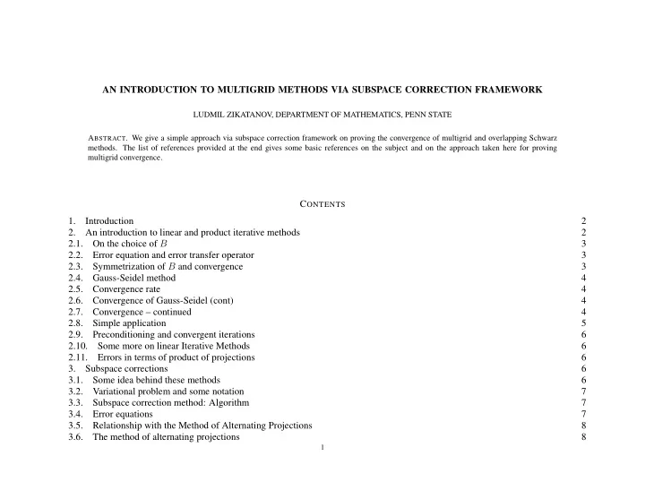
AN INTRODUCTION TO MULTIGRID METHODS VIA SUBSPACE CORRECTION FRAMEWORK LUDMIL ZIKATANOV, DEPARTMENT OF MATHEMATICS, PENN STATE A BSTRACT . We give a simple approach via subspace correction framework on proving the convergence of multigrid and
AN INTRODUCTION TO MULTIGRID METHODS VIA SUBSPACE CORRECTION FRAMEWORK LUDMIL ZIKATANOV, DEPARTMENT OF MATHEMATICS, PENN STATE A BSTRACT . We give a simple approach via subspace correction framework on proving the convergence of multigrid and overlapping Schwarz methods. The list of references provided at the end gives some basic references on the subject and on the approach taken here for proving multigrid convergence. C ONTENTS 1. Introduction 2 2. An introduction to linear and product iterative methods 2 On the choice of B 2.1. 3 2.2. Error equation and error transfer operator 3 Symmetrization of B and convergence 2.3. 3 2.4. Gauss-Seidel method 4 2.5. Convergence rate 4 2.6. Convergence of Gauss-Seidel (cont) 4 2.7. Convergence – continued 4 2.8. Simple application 5 2.9. Preconditioning and convergent iterations 6 2.10. Some more on linear Iterative Methods 6 2.11. Errors in terms of product of projections 6 3. Subspace corrections 6 3.1. Some idea behind these methods 6 3.2. Variational problem and some notation 7 3.3. Subspace correction method: Algorithm 7 3.4. Error equations 7 3.5. Relationship with the Method of Alternating Projections 8 3.6. The method of alternating projections 8 1
4. Convergence of subspace correction methods 9 4.1. Convergence result (preliminaries) 9 4.2. Abstract theorem 10 4.3. Outline of the proof 10 How to estimate c 0 5. 12 5.1. A special decomposition 12 5.2. A multigrid method convergence proof 13 5.3. More general elliptic PDEs 15 5.4. Discretization and subspace splitting 16 5.5. Basic multigrid iteration 16 5.6. Basic facts from Finite element theory 16 5.7. Error estimates 17 5.8. On the addtive methods 17 5.9. Multiplicative overlapping DD-method 18 5.10. Convergence for finite element equations 18 5.11. Convergence via subspace correction framework 18 5.12. Further simplifications: Richardson smoother 19 5.13. Some known results 19 5.14. Stability and convergence 20 Basic references 20 1. I NTRODUCTION 2. A N INTRODUCTION TO LINEAR AND PRODUCT ITERATIVE METHODS • Problem: Find u ∈ R n , such that (1) Au = f, • where A ∈ R n × n is symmetric and positive definite and f ∈ R n is a given right hand side. • Given an initial guess u 0 we find the next iterates u k +1 for k = 0 , 1 , 2 , . . . via the recurrence relation: u k +1 = u k + B ( f − Au k ) , (2) where B ∈ R n × n is some given matrix (an approximate inverse of A ). 2
2.1. On the choice of B . • By convergence, here we mean e k := u − u k , k →∞ � e k � = 0 . lim (3) • For A being SPD, � · � = � · � A . This makes sence, since A defines an inner product on V = R n and also a norm by: � u � 2 ( u, v ) A := � Au, v � ℓ 2 , A = � u, u � A . Let us take u to be the solution to (1). Then by f − Au = 0 we get that u = u + B ( f − Au ) , (4) 2.2. Error equation and error transfer operator. • Subtracting the following two equations u k +1 = u k + B ( f − Au k ) , u = u + B ( f − Au ) it follows that e k = u − u k = ( I − BA ) e k − 1 = . . . = ( I − BA ) k e 0 . • A trivial manipulation then gives that a necessary and sufficient condition for convergence: ρ ( E ) < 1 , with E := I − BA . • But since we would like to have some idea how fast the convergence is, and we also have that A is SPD, we shall use: � e k � A = � ( I − BA ) k e 0 � A ≤ � I − BA � k A � e 0 � A . • Then everything amounts to estimating norm of G := I − BA . that is for any v ∈ V := R n we would like to estimate: A = � ¯ � v � 2 A − � Gv � 2 BAv, v � A , (5) where B := B t + B − B t AB. ¯ (6) 2.3. Symmetrization of B and convergence. • By the following identity: A − � ¯ � Gv � 2 A = � v � 2 BAv, v � A , and we will have convergence, as long as ¯ BA , is positive definite (note that this matrix is symmetric in �· , ·� A inner product. ( ¯ BAv, w ) A = ( A ¯ BAv, w ) = ( Av, ¯ BAw ) = ( v, ¯ BAw ) A • We now take a particular choice of B Gauss-Seidel method and try to estimate the convergence rate 3
2.4. Gauss-Seidel method. • For Gauss-Seidel method we have B := ( D − L ) − 1 , where D is the diagonal of A , and − L is the strict lower triangular part of A . • This means nothing else but that A is written as A = D − L − L t . • Let us compute ¯ B for this choice of B : B t ( B − 1 + B − t − A ) B ¯ B := B t ( D − L + D − L t − D + L + L t ) B = B t DB. = • Hence ¯ B is symmetric and positive definite. and as excersize one can prove that � G � A < 1 , just based on this fact. 2.5. Convergence rate. • As we mentioned before, we are interested in an estimate of � ( I − BA ) � 2 A � G � 2 A = � I − BA � 2 A = sup � v � 2 v � =0 A • Equation (7)gives that ¯ B is invertible. Let us compute ¯ B − 1 : B − 1 = B − 1 D − 1 B − T = ( D − L ) D − 1 ( D − L T ) = A + LD − 1 L T . ¯ 2.6. Convergence of Gauss-Seidel (cont). • Hence yet another expression for ¯ B is below: ¯ B = ( A + LD − 1 L T ) − 1 . • From before A − � ¯ � ( I − BA ) v � 2 A = � v � 2 BAv, v � A . 2.7. Convergence – continued. • After we divide on � v � 2 A and take the sup we obtain that: � ¯ � A ¯ BAv, v � A BAv, v � � ( I − BA ) � 2 A = 1 − inf = 1 − inf � v, v � A � Av, v � v � =0 v � =0 • The expression we have for ¯ B and change of variables w = A 1 / 2 v then can be used to obtain that: � A 1 / 2 ( A + LD − 1 L T ) − 1 A 1 / 2 w, w � � ( I − BA ) � 2 A = 1 − inf . � w, w � w � =0 4
• We use now that for any SPD X λ min ( X ) = 1 /λ max ( X − 1 ) and change back v = A − 1 / 2 w to get that: 1 � ( I − BA ) � 2 A = 1 − . � LD − 1 L T v,v � 1 + sup v � =0 � v,v � A � LD − 1 L T v,v � • Finally if we denote c 0 = sup v � =0 we get that � v,v � A 1 � G � 2 A = 1 − , 1 + c 0 and that is exactly the contraction number in A norm of the Gauss-Seidel iteration. In applications one needs to give an upper bound on c 0 in order to get a convergence result. 2.8. Simple application. h = 1 • Consider A = − D 2 h diag ( − 1 , 2 , − 1) . Because L and D look in a very special way, we have that: N − 1 � � LD − 1 L T v, v � = 1 v 2 i . h 2 i =2 • Therefore for c 0 we obtain: � N − 1 i =2 v 2 i c 0 = sup . h 2 � v, v � A v � =0 � N − 1 i =2 v 2 i • c 0 = sup h 2 � v, v � A v � =0 • The supremum will be achieved for v being the eigenvector corresponding to a minimal eigenvalue of − h 2 D 2 h , just the left boundary point being shifted one h to the right. Hence: 1 c 0 = . 4 sin 2 1 2( N − 1) A = 1 − ch 2 , just by using that for x ∈ [0 , π/ 2] we have that 2 • From here is easy to get that � G � 2 π x ≤ sin x ≤ x , we have that: c 0 ∼ N 2 which gives the desired result. • For − ∆ h the same considerations lead to similar estimate. 5
2.9. Preconditioning and convergent iterations. • There is a difference in the terminology: preconditioning and convergent iterations. • A good preconditioner for A is a matrix B for which κ ( BA ) is uniformly bounded. This does not mean that ρ ( I − BA ) < 1 ! • A good iterator is a matrix B such that � I − BA � ≤ δ < 1 for some norm � · � . Note that if δ is uniformly bounded, then for any eigelue λ ( BA ) we have | λ ( I − BA ) | < 1 ⇒ 1 − δ < | λ ( BA ) | < 1 + δ and hence B is a good preconditioner. • This implication can not be reversed. An example is 2 1 1 B − 1 = diag ( A ) = 2 I. , A = 1 2 1 1 1 2 2.10. Some more on linear Iterative Methods. • In Jacobi B = D − 1 . x ← x + B r ; r := A e = b − A x . • In Gauss Seidel B = ( D − L ) − 1 . • In SOR B = [ ω ( D − L )] − 1 , where ω is selected to minimize ρ ( I − BA ) . 2.11. Errors in terms of product of projections. • If we denote with P k the A -orthogonal projection on span ( e k ) , where φ k is the k -th basis vector: α k = ( Aφ k , v ) / � φ k � 2 P k v = α k ( v ) φ k , A , then ⋆ Jacobi method is an example of additive preconditioner: B = � P k ⋆ Gaus-Seidel and SOR method are product iterative methods, with error transfer operators given by (for Gauss-Seidel ω = 1 ): e k = Ee k , E = ( I − ωP 1 ) . . . ( I − ωP n ) . 3. S UBSPACE CORRECTIONS 3.1. Some idea behind these methods. • The method of subspace corrections is D ivide and Conquer strategy for the solution of a linear equation in a Hilbert space: ⋆ Split the space into sum of subspaces. ⋆ Solve smaller problems on each of the subspaces. ⋆ “Glue up” the solutions of the subspace problems together to get an approximation of the solution in the entire space. • Examples: Gauss-Seidel method, Multigrid method, Schwarz alternating method, Domain decomposition methods ...(just to name a few). 6
Recommend
More recommend
Explore More Topics
Stay informed with curated content and fresh updates.
