AMath 483/583 Lecture 6 Notes: This lecture: NumPy arrays and - - PDF document

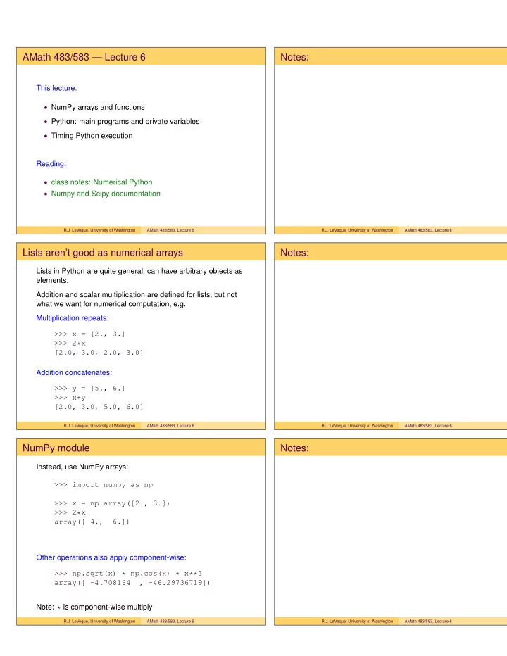
AMath 483/583 — Lecture 6

This lecture:

• NumPy arrays and functions
• Python: main programs and private variables
• Timing Python execution

Reading:

• class notes: Numerical Python
• Numpy and Scipy documentation

R.J. LeVeque, University of Washington AMath 483/583, Lecture 6

Notes:

R.J. LeVeque, University of Washington AMath 483/583, Lecture 6

Lists aren’t good as numerical arrays

Lists in Python are quite general, can have arbitrary objects as elements. Addition and scalar multiplication are defined for lists, but not what we want for numerical computation, e.g. Multiplication repeats: >>> x = [2., 3.] >>> 2*x [2.0, 3.0, 2.0, 3.0] Addition concatenates: >>> y = [5., 6.] >>> x+y [2.0, 3.0, 5.0, 6.0]

R.J. LeVeque, University of Washington AMath 483/583, Lecture 6

Notes:

R.J. LeVeque, University of Washington AMath 483/583, Lecture 6

NumPy module

Instead, use NumPy arrays: >>> import numpy as np >>> x = np.array([2., 3.]) >>> 2*x array([ 4., 6.]) Other operations also apply component-wise: >>> np.sqrt(x) * np.cos(x) * x**3 array([ -4.708164 , -46.29736719]) Note: * is component-wise multiply

R.J. LeVeque, University of Washington AMath 483/583, Lecture 6

Notes:

R.J. LeVeque, University of Washington AMath 483/583, Lecture 6

NumPy arrays

Unlike lists, all elements of an np.array have the same type >>> np.array([1, 2, 3]) # all integers array([1, 2, 3]) >>> np.array([1, 2, 3.]) # one float array([ 1., 2., 3.]) # they’re all floats! Can explicitly state desired data type: >>> x = np.array([1, 2, 3], dtype=complex) >>> print x [ 1.+0.j, 2.+0.j, 3.+0.j] >>> (x + 1.j) * 2.j array([-2.+2.j, -2.+4.j, -2.+6.j])

R.J. LeVeque, University of Washington AMath 483/583, Lecture 6

Notes:

R.J. LeVeque, University of Washington AMath 483/583, Lecture 6

NumPy arrays for vectors and matrices

>>> A = np.array([[1.,2], [3,4], [5,6]]) >>> A array([[ 1., 2.], [ 3., 4.], [ 5., 6.]]) >>> A.shape (3, 2) >>> A.T array([[ 1., 3., 5.], [ 2., 4., 6.]]) >>> x = np.array([1., 1.]) >>> x.T array([ 1., 1.])

R.J. LeVeque, University of Washington AMath 483/583, Lecture 6

Notes:

R.J. LeVeque, University of Washington AMath 483/583, Lecture 6

NumPy arrays for vectors and matrices

>>> A array([[ 1., 2.], [ 3., 4.], [ 5., 6.]]) >>> x array([ 1., 1.]) >>> np.dot(A,x) # matrix-vector product array([ 3., 7., 11.]) >>> np.dot(A.T, A) # matrix-matrix product array([[ 35., 44.], [ 44., 56.]])

R.J. LeVeque, University of Washington AMath 483/583, Lecture 6

Notes:

R.J. LeVeque, University of Washington AMath 483/583, Lecture 6

NumPy matrices for vectors and matrices

For Linear algebra, may instead want to use numpy.matrix: >>> A = np.matrix([[1.,2], [3,4], [5,6]]) >>> A matrix([[ 1., 2.], [ 3., 4.], [ 5., 6.]]) Or, Matlab style (as a string that is converted): >>> A = np.matrix("1.,2; 3,4; 5,6") >>> A matrix([[ 1., 2.], [ 3., 4.], [ 5., 6.]])

R.J. LeVeque, University of Washington AMath 483/583, Lecture 6

Notes:

R.J. LeVeque, University of Washington AMath 483/583, Lecture 6

NumPy matrices for vectors and matrices

Note: vectors are handled as matrices with 1 row or column: >>> x = np.matrix("4.;5.") >>> x matrix([[ 4.], [ 5.]]) >>> x.T matrix([[ 4., 5.]]) >>> A*x matrix([[ 14.], [ 32.], [ 50.]]) But note that indexing into x requires two indices: >>> print x[0,0], x[1,0] 4.0 5.0

R.J. LeVeque, University of Washington AMath 483/583, Lecture 6

Notes:

R.J. LeVeque, University of Washington AMath 483/583, Lecture 6

Which to use, array or matrix?

For linear algebra matrix may be easier (and more like Matlab), but vectors need two subscripts! For most other uses, arrays more natural, e.g. >>> x = np.linspace(0., 3., 100) # 100 points >>> y = x**5 - 2.*sqrt(x)*cos(x) # 100 values >>> plot(x,y) np.linspace returns an array, which is what is needed here. We will always use arrays. See http://www.scipy.org/NumPy_for_Matlab_Users

R.J. LeVeque, University of Washington AMath 483/583, Lecture 6

Notes:

R.J. LeVeque, University of Washington AMath 483/583, Lecture 6

Rank of an array

The rank of an array is the number of subscripts it takes: >>> A = np.ones((4,4)) >>> A array([[ 1., 1., 1., 1.], [ 1., 1., 1., 1.], [ 1., 1., 1., 1.], [ 1., 1., 1., 1.]]) >>> np.rank(A) 2 Warning: This is not the rank of the matrix in the linear algebra sense (dimension of the column space)!

R.J. LeVeque, University of Washington AMath 483/583, Lecture 6

Notes:

R.J. LeVeque, University of Washington AMath 483/583, Lecture 6

Rank of an array

Scalars have rank 0: >>> z = np.array(7.) >>> z array(7.0) NumPy arrays of any dimension are supported, e.g. rank 3: >>> T = np.ones((2,2,2)) >>> T array([[[ 1., 1.], [ 1., 1.]], [[ 1., 1.], [ 1., 1.]]]) >>> T[0,0,0] 1.0

R.J. LeVeque, University of Washington AMath 483/583, Lecture 6

Notes:

R.J. LeVeque, University of Washington AMath 483/583, Lecture 6

Linear algebra with NumPy

>>> A = np.array([[1., 2.], [3, 4]]) >>> A array([[ 1., 2.], [ 3., 4.]]) >>> b = np.dot(A, np.array([8., 9.])) >>> b array([ 26., 60.]) Now solve Ax = b: >>> from numpy.linalg import solve >>> solve(A,b) array([ 8., 9.])

R.J. LeVeque, University of Washington AMath 483/583, Lecture 6

Notes:

R.J. LeVeque, University of Washington AMath 483/583, Lecture 6

Eigenvalues

>>> from numpy.linalg import eig >>> eig(A) # returns a tuple (evals,evecs) (array([-0.37228132, 5.37228132]), array([[-0.82456484, -0.41597356], [ 0.56576746, -0.90937671]])) >>> evals, evecs = eig(A) # unpacks tuple >>> evals array([-0.37228132, 5.37228132]) >>> evecs array([[-0.82456484, -0.41597356], [ 0.56576746, -0.90937671]])

R.J. LeVeque, University of Washington AMath 483/583, Lecture 6

Notes:

R.J. LeVeque, University of Washington AMath 483/583, Lecture 6

Quadrature (numerical integration)

Estimate 2

0 x2 dx = 8/3:

>>> from scipy.integrate import quad >>> def f(x): ... return x**2 ... >>> quad(f, 0., 2.) (2.666666666666667, 2.960594732333751e-14) returns (value, error estimate). Other keyword arguments to set error tolerance, for example.

R.J. LeVeque, University of Washington AMath 483/583, Lecture 6

Notes:

R.J. LeVeque, University of Washington AMath 483/583, Lecture 6

Lambda functions

In the last example, f is so simple we might want to just include its definition directly in the call to quad. We can do this with a lambda function: >>> f = lambda x: x**2 >>> f(4) 16 This defines the same f as before. But instead we could do: >>> quad(lambda x: x**2, 0., 2.) (2.666666666666667, 2.960594732333751e-14)

R.J. LeVeque, University of Washington AMath 483/583, Lecture 6

Notes:

R.J. LeVeque, University of Washington AMath 483/583, Lecture 6

“Main program” in a Python module

Python modules often end with a section that looks like: if __name__ == "__main__": # some code This code is not executed if the file is imported as a module,

• nly if it is run as a script, e.g. by...

$ python filename.py >>> execfile("filename.py") In[1]: run filename.py (See $UWHPSC/lectures/lecture6/mysqrt.py)

R.J. LeVeque, University of Washington AMath 483/583, Lecture 6

Notes:

R.J. LeVeque, University of Washington AMath 483/583, Lecture 6

Timing Python code

Demo in $UWHPSC/lectures/lecture6

R.J. LeVeque, University of Washington AMath 483/583, Lecture 6

Notes:

R.J. LeVeque, University of Washington AMath 483/583, Lecture 6