AMath 483/583 Lecture 26 Outline: Monte Carlo methods Random - PowerPoint PPT Presentation
AMath 483/583 Lecture 26 Outline: Monte Carlo methods Random number generators Monte Carlo integrators Random walk solution of Poisson problem R.J. LeVeque, University of Washington AMath 483/583, Lecture 26 Announcements
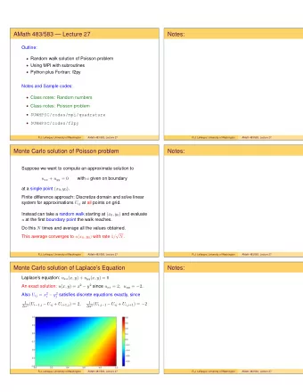
AMath 483/583 — Lecture 26 Outline: • Monte Carlo methods • Random number generators • Monte Carlo integrators • Random walk solution of Poisson problem R.J. LeVeque, University of Washington AMath 483/583, Lecture 26
Announcements Part of Final Project will be available tomorrow. R.J. LeVeque, University of Washington AMath 483/583, Lecture 26
Announcements Part of Final Project will be available tomorrow. No Class on Monday, June 2 R.J. LeVeque, University of Washington AMath 483/583, Lecture 26
Announcements Part of Final Project will be available tomorrow. No Class on Monday, June 2 Wednesday, June 4: Please come for course evaluations. R.J. LeVeque, University of Washington AMath 483/583, Lecture 26
AMath 483/583 — Lecture 26 Outline: • Monte Carlo methods • Random number generators • Monte Carlo integrators • Random walk solution of Poisson problem R.J. LeVeque, University of Washington AMath 483/583, Lecture 26
Monte Carlo Methods Computational methods that use random (or pseudo-random) sampling to obtain numerical approximations. Originally developed developed in 1940’s at Los Alamos for neutron diffusion problems. R.J. LeVeque, University of Washington AMath 483/583, Lecture 26
Monte Carlo methods Examples: • Approximate a definite integral by sampling the integrand at random points (rather than on a regular grid, as with Trapezoid or Simpson). • Random walk solution to a Poisson problem • Given a probability distribution of inputs to some problem, estimate probability distribution of output. Sensitivity analysis Uncertainty quantification • Simulate processes that have random data or forcing. R.J. LeVeque, University of Washington AMath 483/583, Lecture 26
Classical quadrature Midpoint rule in 1 dimension: � b n � f ( x ) dx ≈ h f ( x i ) a i =1 There are n terms in sum and accuracy is O ( h 2 ) = O (1 /n 2 ) R.J. LeVeque, University of Washington AMath 483/583, Lecture 26
Classical quadrature Midpoint rule in 1 dimension: � b n � f ( x ) dx ≈ h f ( x i ) a i =1 There are n terms in sum and accuracy is O ( h 2 ) = O (1 /n 2 ) Midpoint rule in 2 dimensions: � b 2 � b 1 n n g ( x [ i ] 1 , x [ j ] g ( x 1 , x 2 ) dx 1 dx 2 ≈ h 2 � � 2 ) a 2 a 1 j =1 i =1 There are N = n 2 terms in sum and accuracy is O ( h 2 ) = O (1 /n 2 ) = O (1 /N ) R.J. LeVeque, University of Washington AMath 483/583, Lecture 26
Classical quadrature Midpoint rule in 20 dimensions: � b 20 � b 2 � b 1 g ( x 1 , x 2 , . . . , x 20 ) dx 1 dx 2 · · · dx 20 · · · a 20 a 2 a 1 n n n g ( x [ i ] 1 , x [ j ] 2 , . . . , x [ k ] ≈ h 20 � � � 20 ) · · · k =1 j =1 i =1 There are N = n 20 terms in sum and accuracy is O ( h 2 ) = O (1 /n 2 ) = O ((1 /N ) 1 / 10 ) R.J. LeVeque, University of Washington AMath 483/583, Lecture 26
Classical quadrature Midpoint rule in 20 dimensions: � b 20 � b 2 � b 1 g ( x 1 , x 2 , . . . , x 20 ) dx 1 dx 2 · · · dx 20 · · · a 20 a 2 a 1 n n n g ( x [ i ] 1 , x [ j ] 2 , . . . , x [ k ] ≈ h 20 � � � 20 ) · · · k =1 j =1 i =1 There are N = n 20 terms in sum and accuracy is O ( h 2 ) = O (1 /n 2 ) = O ((1 /N ) 1 / 10 ) Note: with only n = 10 points in each direction, N = 10 20 . On 1 GFlop computer, would take 10 11 seconds > 3000 years to compute sum and get accuracy ≈ 1 /n 2 = 0 . 01 . R.J. LeVeque, University of Washington AMath 483/583, Lecture 26
Classical quadrature Midpoint rule in 20 dimensions: � b 20 � b 2 � b 1 g ( x 1 , x 2 , . . . , x 20 ) dx 1 dx 2 · · · dx 20 · · · a 20 a 2 a 1 n n n g ( x [ i ] 1 , x [ j ] 2 , . . . , x [ k ] ≈ h 20 � � � 20 ) · · · k =1 j =1 i =1 There are N = n 20 terms in sum and accuracy is O ( h 2 ) = O (1 /n 2 ) = O ((1 /N ) 1 / 10 ) Note: with only n = 10 points in each direction, N = 10 20 . On 1 GFlop computer, would take 10 11 seconds > 3000 years to compute sum and get accuracy ≈ 1 /n 2 = 0 . 01 . Also each evaluation of g might be expensive! R.J. LeVeque, University of Washington AMath 483/583, Lecture 26
High dimensions might arise from many parameters... Example: Solve chemical kinetics equations u ′ ( t ) = F ( u ( t )) for system with 20 reacting species and “mass action kinetics” in a stirred tank (so concentrations vary with time but not space). R.J. LeVeque, University of Washington AMath 483/583, Lecture 26
High dimensions might arise from many parameters... Example: Solve chemical kinetics equations u ′ ( t ) = F ( u ( t )) for system with 20 reacting species and “mass action kinetics” in a stirred tank (so concentrations vary with time but not space). Need initial concentrations, e.g. u 1 (0) = x 1 , u 2 (0) = x 2 , . . . , u 20 (0) = x 20 . Suppose we want to determine u 15 ( T ) = g ( x 1 , x 2 , . . . , x 20 ) . R.J. LeVeque, University of Washington AMath 483/583, Lecture 26
High dimensions might arise from many parameters... Example: Solve chemical kinetics equations u ′ ( t ) = F ( u ( t )) for system with 20 reacting species and “mass action kinetics” in a stirred tank (so concentrations vary with time but not space). Need initial concentrations, e.g. u 1 (0) = x 1 , u 2 (0) = x 2 , . . . , u 20 (0) = x 20 . Suppose we want to determine u 15 ( T ) = g ( x 1 , x 2 , . . . , x 20 ) . Suppose initial conditions are not known exactly, but we know a 1 ≤ x 1 ≤ b 2 , . . . , a 20 ≤ x 20 ≤ b 20 . R.J. LeVeque, University of Washington AMath 483/583, Lecture 26
High dimensions might arise from many parameters... Example: Solve chemical kinetics equations u ′ ( t ) = F ( u ( t )) for system with 20 reacting species and “mass action kinetics” in a stirred tank (so concentrations vary with time but not space). Need initial concentrations, e.g. u 1 (0) = x 1 , u 2 (0) = x 2 , . . . , u 20 (0) = x 20 . Suppose we want to determine u 15 ( T ) = g ( x 1 , x 2 , . . . , x 20 ) . Suppose initial conditions are not known exactly, but we know a 1 ≤ x 1 ≤ b 2 , . . . , a 20 ≤ x 20 ≤ b 20 . We might want to estimate the expected value of u 15 ( T ) � b 20 � b 2 � b 1 1 = · · · g ( x 1 , x 2 , . . . , x 20 ) dx 1 dx 2 · · · dx 20 . Volume a 20 a 2 a 1 R.J. LeVeque, University of Washington AMath 483/583, Lecture 26
Classical quadrature N = 100 points in two space dimensions for Midpoint: � b 2 � b 1 n n g ( x [ i ] 1 , x [ j ] g ( x 1 , x 2 ) dx 1 dx 2 ≈ h 2 � � 2 ) a 2 a 1 j =1 i =1 R.J. LeVeque, University of Washington AMath 483/583, Lecture 26
Monte Carlo integration N = 100 random points in the same 2-dimensional region: � b 2 � b 1 N g ( x 1 , x 2 ) dx 1 dx 2 ≈ V g ( x [ k ] 1 , x [ k ] � 2 ) N a 2 a 1 k =1 V = ( b 2 − a 2 )( b 1 − a 1 ) is volume. R.J. LeVeque, University of Washington AMath 483/583, Lecture 26
Monte Carlo integration √ Accuracy: With N random points, error is O (1 / N ) . This is true independent of the number of dimensions! R.J. LeVeque, University of Washington AMath 483/583, Lecture 26
Monte Carlo integration √ Accuracy: With N random points, error is O (1 / N ) . This is true independent of the number of dimensions! In 20 dimensions, if g is smooth than can expect error ≈ 0 . 01 with N = 10000 . (vs. N = 10 20 for Midpoint.) R.J. LeVeque, University of Washington AMath 483/583, Lecture 26
Log-log plot of errors with Monte Carlo √ N = N − 1 / 2 . Black line: 1 / √ ⇒ log( E ( N )) = log( C ) − 1 Note that E ( N ) = C/ N = 2 log( N ) Red points: For an integral in 2 dimensions Blue points: For an integral in 20 dimensions R.J. LeVeque, University of Washington AMath 483/583, Lecture 26
Pseudo-Random number generators Hard to generate a truly random number on the computer. Instead generally use pseudo-random number generators that produce a sequence of numbers by some deterministic formula, but designed so that numbers generated are approximately distributed according to desired distribution. R.J. LeVeque, University of Washington AMath 483/583, Lecture 26
Pseudo-Random number generators Hard to generate a truly random number on the computer. Instead generally use pseudo-random number generators that produce a sequence of numbers by some deterministic formula, but designed so that numbers generated are approximately distributed according to desired distribution. Linear congruential generator: X n +1 = aX n + c mod m e.g. from Numerical Recipes : a = 1664525 , c = 1013904223 , m = 2 32 Requires a seed X 0 to get started. R.J. LeVeque, University of Washington AMath 483/583, Lecture 26
Pseudo-Random number generators In Python: Plot of 100 random points was generated using... from numpy.random import RandomState random_generator = RandomState(seed=55) r = random_generator.uniform(0., 1., size=200) plot(r[::2],r[1::2],’bo’) R.J. LeVeque, University of Washington AMath 483/583, Lecture 26
Pseudo-Random number generators In Python: Plot of 100 random points was generated using... from numpy.random import RandomState random_generator = RandomState(seed=55) r = random_generator.uniform(0., 1., size=200) plot(r[::2],r[1::2],’bo’) Initializing with seed=None will use a “random” seed. Specifying a seed makes it possible to reproduce the same results later. R.J. LeVeque, University of Washington AMath 483/583, Lecture 26
Recommend
More recommend
Explore More Topics
Stay informed with curated content and fresh updates.
