* Alternative technique not covered in this class Multivariate - PowerPoint PPT Presentation

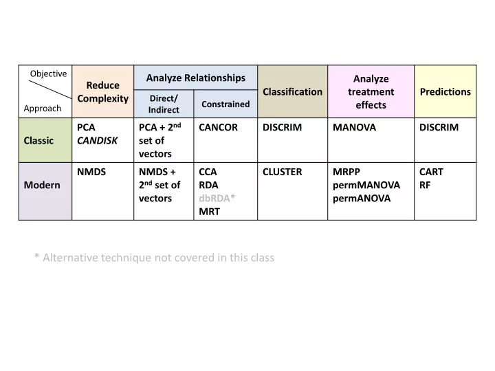
Objective Analyze Relationships Analyze Reduce Classification treatment Predictions Complexity Direct/ Constrained effects Approach Indirect PCA + 2 nd PCA CANCOR DISCRIM MANOVA DISCRIM Classic CANDISK set of vectors NMDS NMDS + CCA CLUSTER MRPP CART 2 nd set of Modern RDA permMANOVA RF vectors dbRDA* permANOVA MRT * Alternative technique not covered in this class

Multivariate Fundamentals: Prediction Classification and Regression Trees (CART) MCMT>=-30.85 MCMT< -30.85 0.674 n=103 MCMT>=-25.8 MCMT< -25.8 0.534 4.15 n=99 n=4 MWMT< 16.45 MWMT>=16.45 0.172 1.2 n=64 n=35 0.601 2.92 n=26 n=9 Error : 0.214 CV Error : 0.412 SE : 0.122

Objective: Determine what drives relationships between response and predictor variables in more detail (unimodal or bimodal relationships) CART is Univariate MRT is Multivariate We aim to answer: “ What distinguishes my groups within my predictor variables?” Classification and Regression Trees can use both categorical and continuous numeric response variables – If response is categorical a classification tree is used to identify the "class" within which a target variable would likely fall into – If response is continuous a regression tree is used to predict it's value – We cover both in Lab 8 Also referred to as decision trees If we can specifically determine what drives a relationship, we can use that information to predict a response under new conditions

The math behind CART (and MRT in multivariate space) Consider: “ What drives species frequency? ” Species Frequency MAT Try and look at a ordination 1 2 3 4 5 6 7 MAT °C When the relationship is not linear, ordinations do not work out cleanly E.g. Species are both low species frequency, but have very different MAT thresholds, so where do I draw the arrow to capture this information?

The math behind CART < 2°C ≥ 2 °C Node Species Frequency < 6°C ≤ 6 °C Leaf 1 2 3 4 5 6 7 High Low Low MAT °C Alternatively we can build a decision tree to better define and illustrate the species frequency-temperature relationship Think of this as a cluster analysis where splits are constrained by environmental variables (like in Constrained Gradient Analysis)

The math behind CART CART is an iterative top-down process that aims to minimize within group variation To start the tree, CART empirically investigating various thresholds in various predictor variables to find the first split in the response variable dataset that minimizing variation within groups (like Cluster Analysis) However unlike Cluster Analysis, the external variables (the predictors) are imposed as a constraint to create the clusters E.g. Using environmental thresholds to create clusters of inventory plots with similar species composition The process then repeats for the two sub-groups, until no significant amount of additional variation ca be explained by further splits

CART in R There are other R packages that build univariate Classification (categorical) and Regression (numeric) Trees – e.g. tree and rpart To simplify for this class we will use the package mvpart which is primarily designed to execute Multivariate Regression Trees (MRT), but can handle CART as well Vector of response variable (univariate) Equation of Predictors : To run CART you need Variable1 include single predictor to install the mvpart Variable1+Variable2 include multiple predictors package Data table of your predictor variables E.g. Environmental Variables CART in R: library(mvpart) mvpart(ResponseVariable,EquationOfPredictors,data=predictorData, (mvpart package) xv= " p " , all.leaves=T) Specifying xv= " p “ allows you to Turn on the option all.leaves=T to generate the number interactively pick the tree size you of observations and the average frequency at each node want to generate and leaf

CART in R Picking the tree size is a good option to specify because it allows you to pick the best tree which includes well supported splits that explain a significant portion of the variation By specifying xv= " p " R will generate a screen-plot for decision guidance Size of tree – number of splits Green line – equivalent to “ variance explained by each split ” statistic Red line – minimum relative error corresponding to minimum variance explained plus one standard error Blue line – tree performance associated with splits Orange mark – well supported splits that explain sufficient variation Red mark – reasonably well supported splits explaining some additional variation Cross-validation prediction You should pick a tree size under the red line, between the orange and red marks The bigger the tree the bigger the breakdown among data points – you have to determine how far you want to breakdown your data (you might go too far and remove groupings that you want) If you don’t specify xv= " p " in your mvpart statement then the tree size at the orange mark will be used

CART in R R will output a regression tree We build a model to look at a single species frequency with 5 predictor variables Predictor variable associated MCMT>=-30.85 MCMT< -30.85 with data split 0.674 n=103 The average species frequency for the group MCMT>=-25.8 MCMT< -25.8 0.534 4.15 (e.g. 4.15%) n=99 n=4 The number of MWMT< 16.45 MWMT>=16.45 Errors associated with the tree size: 0.172 1.2 data points that n=64 n=35 fall into this group Error: Residual error how much variation is (e.g. n = 64 data points) not explained by the tree CV Error: Summarized cross-validated relative 0.601 2.92 n=26 n=9 error for all predictors (zero for perfect predictor to close to one for a poor predictor) Error : 0.214 CV Error : 0.412 SE : 0.122 You want small values for both! If you have a big tree the tree image will be crowded (this is a problem in mvpart), so save the image as a enhanced metafile (option in the save) You can then import the emf file into Powerpoint, ungroup it twice and move the labels around to make the image more legible and publishable

CART in R We build a model to look at a single species frequency with 5 predictor variables The variation explained by each split For each node (and leaf) details about the split are provided: • Number of observations used • Mean of the group • Mean square error of the group • How many observations are divided into each side of the split • Primary splits (potential alternative predictors) Improvement values indicate how much variation would be explained if that split was based on an alternative variable If the improve value at a split is the same for a different predictor variable, the alternative predictor variable could be used to explain the groupings

Multivariate Fundamentals: Prediction Multivariate Regression Trees (MRT) ABIELAS MCMT>=-14.85 MCMT< -14.85 PICEENG PINUCON PICEGLA 810 : n=136 POPUTRE PINUBAN MAT>=0.6 MAT< 0.6 MAT>=-0.4 MAT< -0.4 334 : n=80 303 : n=56 MWMT< 16 MWMT>=16 MWMT< 15.9 MWMT>=15.9 MAT< -1.3 MAT>=-1.3 MSP< 304.5 MSP>=304.5 71.1 : n=64 154 : n=16 158 : n=32 0.487 : n=8 6.12 : n=16 9.93 : n=40 13.8 : n=24 MSP< 332 MSP>=332 58 : n=24 0.791 : n=8 0.0026 : n=8 0.848 : n=8 10.5 : n=16 0.495 : n=8 Error : 0.053 CV Error : 0.102 SE : 0.0313

Objective: Determine what drives relationships between multiple response and predictor variables in more detail (unimodal or bimodal relationships ) Just like CART, but multivariate space We aim to answer: “ What distinguishes my groups within my predictor variables?” Like CART, MRT can use both categorical and continuous numeric response variables If we can specifically determine what drives a relationship, we can use that information to predict a response under new conditions

MRT in R Matrix of response variables E.g: Frequencies for multiple species Equation of Predictors: Variable1 include single predictor To run CART you need Variable1+Variable2 include multiple predictors to install the mvpart package Data table of your predictor variables E.g. Environmental Variables MRT in R: library(mvpart) mvpart(ResponseMatrix,EquationOfPredictors,data=predictorData, (mvpart package) xv= " p " , all.leaves=T) Specifying xv= " p “ allows you to Turn on the option all.leaves=T to generate the number interactively pick the tree size you of observations and the average frequency at each node want to generate and leaf To make the MRT output easier to interpret, response variables should be normalized prior to conducting the MRT analysis