Aggregate Demand and Aggregate Supply 2013 Outline Friday 14 th : - PowerPoint PPT Presentation
Aggregate Demand and Aggregate Supply 2013 Outline Friday 14 th : Chapter 16 (AS-AD, demand policies) 1. Monday 18 th 2. Bas Jacobs (45 to 60 minutes interactive lecture on current crisis) Chapter 17 (debt and stabilization policies)
Aggregate Demand and Aggregate Supply 2013
Outline Friday 14 th : Chapter 16 (AS-AD, demand policies) 1. Monday 18 th 2. Bas Jacobs (45 to 60 minutes interactive lecture on current crisis) Chapter 17 (debt and stabilization policies) Wednesday 20 th : end of Chapter 17 + Chapter 14/15 3. Friday 22 nd : end of Chapter 15 + solutions to mock exam 4.
Introduction The big picture Short run Medium run Long run
Introduction AS-AD in the short run Aggregate demand and aggregate supply Phillips curve & Okun’s law (Chapter AS 12) Inflation Equilibrium on the goods and money market, IS-TR (Chapter 10) AD Output gap
Introduction AS-AD in the long run LAS Inflation LAD Output gap
Literature for AS-AD model Lecture notes + pdf « Notes Chapter 13» Burda & Wyplosz: 13.3.1 The Fisher equation 13.3.2 The long-run AD curve 13.3.6 Monetary Policy 13.4 – 13.4.3 How to use the AS-AD framework In the lecture: no international capital markets in this framework (we don’t talk explicitly about exchange rate, but implicitely we assume a flexible exchange rate regime). Skip the details on the differences between fixed and flexible exchange rate. Model presented here based on Mankiw, Macroeconomics , 7 th edition of the international edition, Chapter 14, mainly section 14.3 and 14.4
Outline Introduction 1. The Fisher equation 2. Recall: Phillips curve, expectations and aggregate supply 3. Aggregate demand 4. Long run 1. Short run 2. Using the AD-AS framework: Explaining fluctuations 5. Supply shocks 1. Demand shocks 2. Monetary policy 3. The role of Policies 4.
Introduction Keeping track of time We use a dynamic model of aggregate supply and demand. Therefore: we need to introduce the time dimension The subscript “ t ” denotes the time period, e.g . Y t = real GDP in period t Y t -1 = real GDP in period t – 1 Y t +1 = real GDP in period t + 1 We can think of time periods as years, e .g ., if t = 2008, then Y t = Y 2008 = real GDP in 2008 Y t -1 = Y 2007 = real GDP in 2007 Y t +1 = Y 2009 = real GDP in 2009
Introduction The model’s variables and parameters Endogenous variables (we see how these evolve over time): Y t : output 2. … what happens to those? π t : inflation r t : real interest rate i t : nominal interest rate ~ : underlying inflation t Shows us how last period’s events influences today’s outcome Exogenous variables (determined outside of our model) : : trend output Y 1. If we change one of these… : inflation target by CB Demand shocks: G, T, wealth, consumer confidence… s t : Supply shocks
2. The Fisher equation The Fisher equation Central bank sets the nominal interest rate i : i i a bY gap gap Distinction between nominal and real interest rate e r i t t t t r t : real intrest rate - relevant for spending decisions i t : nominal intrest rate - relevant for money market e : inflation that I expect today will happen between today (year t ) t t and tomorrow (t+1) Notation: π t : ex-post observed inflation between year t and year t+1 π t-1 : observed inflation between last period (t-1) and today (t)
2. The Fisher equation The Fisher equation Example: i = 8%, π t e =10% r=? r =0,08-0,10= -0,02 Your money will buy 2% fewer goods Lender: prefers low inflation Borrower: prefers high inflation r i t t t r = only observable ex post CB fixes the nominal interest rate and long run inflation expectations
3. Recall: Phillips curve Phillips curve ~ Phillips curve: bU s t t gap t Short run: Trade-off between inflation and unemployment possible IF no supply shocks Inflation Long run underlying inflation constant U n constant. ~ Long-run: 2 B A ~ ~ Short run & s 0 U U t t t t 1 Phillips curves No trade-off possible between unemployment and inflation U Unemployment
3. Recall: Phillips curve Underlying inflation ~ Underlying inflation : expected inflation Two components Backward looking component ( π t-1 ) Forward looking component (long run inflation rate) For the moment, we assume adaptive expectations. Adaptive expectations: focus on backward looking component Realistic when π relatively stable ~ e t t t t 1 Later & Chapter 16: Incorporate again the forward looking component: Inflation target fixed by the central bank
3. Recall: Phillips curve From the Phillips curve to aggregate supply (a) Phillips curve Inflation ~ bU gap s Aggregate supply ~ aY gap s Inflation Unemployment U (b) Okun‘s law Unemployment U hY gap gap U Y Output Y Output
3. Recall: Philips curve Aggregate supply curve Aggregate supply curve describes, for each given level of inflation, π , the quantity of output firms are willing to supply, Y ~ Long run AS aY s Inflation t t gap t Medium run: upward sloping, long run: vertical ~ Derived from the Phillips curve: B 2 A ~ Short Inflation unemployment 1 run AS Shift of AS (and Phillips) curve: • Change in underlying inflation • Supply shock, s ≠0 Y Output • (Change in natural U or natural Y)
4. Aggregate demand Aggregate demand Aggregate demand curve all the combinations of output and inflation such that the market for goods is in equilibrium (IS) the money market is in equilibrium (TR ) To draw the aggregate demand curve: How does the equilibrium on the goods and money markets change when prices change? 1. Long run AD curve 2. Short run AD curve Here: closed or big and open economy (!!DIFFERENT from Ch. 13 of Burda & Wyplosz!!) we do not worry about the exchange rate here Framework here: based on Mankiw, Macroeconomics , 7 th edition of the international edition, Chapter 14
4.1 Aggregate demand – Long run The model’s long run equilibrium We know (from the LAS curve) that in the long run ~ Y Y t t t t Intersection of LAS and LAD curve: Long run equilibrium of the economy What determines inflation in the long run? CB fixes the inflation target and thus long run inflation It follows: ~ t t r i t Real economy gives natural level of real interest rate: r r
4.1 Aggregate demand – Long run The aggregate demand curve in the long run Taylor rule : i i a bY , where i r gap gap Central bank chooses a target for the long run inflation Inflation independent from output Inflation LAD = target inflation frate Output gap
4.2 Aggregate demand – Short run Aggregate demand curve in the short run Deriving the short run AD curve: How does a change in prices affect the equilibrium in the IS- TR model? Taylor rule: i i a bY gap gap Interest rate responds not only to changes in Y but also to changes in π ECB: a = 1.5 i ↑ if π gap >0. (note: i increases by more than π gap !) r increases also (i – π = r) When inflation changes shift of TR curve If inflation raises, for every level of output, the interest rate will be higher, so the TR curve shifts up
4.2 Aggregate demand – Short run Taylor rule and inflation How does the CB change i when inflation increases? TR‘ i i i a bY gap gap TR i i i a ( ) bY gap 0 Y gap π a π i i a bY gap This constant term will change, when π i when changes
4.2 Aggregate demand – Short run Drawing the short run AD curve At point A: and Y Y i i Along TR is held constant Interest rate TR at . A i We start Output gap 0 from long-run Rate of inflation equilibrium, where Y 0 A gap and . Output gap 0
4.2 Aggregate demand – Short run Drawing the short run AD curve i i a bY gap gap Interest rate TR ´ IS TR A ´ With π : TR TR’. A Nominal and real interest rate Output gap 0 Investment , Y Rate of inflation A ´ Question: Why is r automatically A here, after the ECB increases i according to AD the Taylor rule ( a = 1.5)? Output gap 0
4.2 Aggregate demand – Short run The short run AD curve AD determined by changes in the IS-TR equilibrium due to change in inflation AD slopes downward : When inflation rises, the central bank π raises the (real) interest rate, reducing the demand for goods & services. AD curve shifts in response to changes in • the inflation target (↑ shifts AD to the right) AD t • demand shocks ( ε = changes in Y gap G, T, wealth, …) (↑ in demand shift to the right) Y gap A ( ) B
5. Using the AD-AS framework: Explaining fluctuations AS-AD LAS AS Inflation LAD AD 0 Output gap
Recommend
More recommend
Explore More Topics
Stay informed with curated content and fresh updates.
