Administrivia Students are 75% EE, 25% CS. Lecture 2 Top three - PowerPoint PPT Presentation
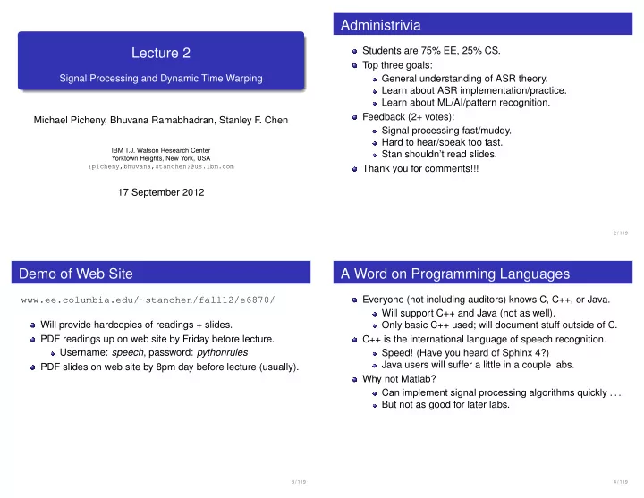
Administrivia Students are 75% EE, 25% CS. Lecture 2 Top three goals: Signal Processing and Dynamic Time Warping General understanding of ASR theory. Learn about ASR implementation/practice. Learn about ML/AI/pattern recognition. Feedback
Administrivia Students are 75% EE, 25% CS. Lecture 2 Top three goals: Signal Processing and Dynamic Time Warping General understanding of ASR theory. Learn about ASR implementation/practice. Learn about ML/AI/pattern recognition. Feedback (2+ votes): Michael Picheny, Bhuvana Ramabhadran, Stanley F. Chen Signal processing fast/muddy. Hard to hear/speak too fast. IBM T.J. Watson Research Center Stan shouldn’t read slides. Yorktown Heights, New York, USA {picheny,bhuvana,stanchen}@us.ibm.com Thank you for comments!!! 17 September 2012 2 / 119 Demo of Web Site A Word on Programming Languages Everyone (not including auditors) knows C, C++, or Java. www.ee.columbia.edu/~stanchen/fall12/e6870/ Will support C++ and Java (not as well). Will provide hardcopies of readings + slides. Only basic C++ used; will document stuff outside of C. PDF readings up on web site by Friday before lecture. C++ is the international language of speech recognition. Username: speech , password: pythonrules Speed! (Have you heard of Sphinx 4?) Java users will suffer a little in a couple labs. PDF slides on web site by 8pm day before lecture (usually). Why not Matlab? Can implement signal processing algorithms quickly . . . But not as good for later labs. 3 / 119 4 / 119
Review: A Very Simple Speech Recognizer Today’s Lecture Training data: audio sample A w for every word w ∈ vocab. w ∗ = arg min distance ( A test , A w ) Given test sample A test , pick word w ∗ : w ∈ vocab w ∗ = arg min distance ( A test , A w ) w ∈ vocab signal processing — Extract features from audio . . . So simple distance measure works. dynamic time warping — Handling time/rate variation in the distance measure. 5 / 119 6 / 119 Part I Goals of Feature Extraction Capture essential information for word identification. Signal Processing Make it easy to factor out irrelevant information. e.g. , long-term channel transmission characteristics. Compress information into manageable form. Figures in this section from [Holmes] , [HAH] or [R+J] unless indicated otherwise. 7 / 119 8 / 119
What Has Actually Worked? Concept: The Frame 1 1950s–1960s — Analog filterbanks. Raw 16kHz input: sample every 16000 sec. 1970s — Linear Predictive Coding (LPC). What should output look like? Point: speech phenomena aren’t that short. 1980s — LPC Cepstra. 1 e.g. , output frame of features every, say, 100 sec . . . 1990s — Mel-Scale Cepstral Coefficients (MFCC) and 1 Describing what happened in that 100 sec. Perceptual Linear Prediction (PLP). How wide should feature vector be? 2000s — Posteriors and multistream combinations. Empirically: 40 or so. e.g. , 1s of audio: 16000 × 1 nums in ⇒ 100 × 40 nums out. 9 / 119 10 / 119 LPC Ceptra, MFCC, and PLP: The Basic Idea What is a Short-Term Spectrum? For each frame: Extract out window of samples for that frame. Step 1: Compute short-term spectrum. Compute energy at each frequency using discrete Fourier Step 2: From spectrum, compute cepstrum . transform. Step 3: Profit! Look at signal as decomposition of its frequency Each method does these steps differently. components. LPC inspired by human production. Lots more gory details in next section. MFCC, PLP inspired by human perception. 11 / 119 12 / 119
Why the Short-Term Spectrum? What is a Cepstrum? Matches human perception/physiology? (Inverse) Fourier transform of . . . This sounds like what the cochlea is doing? Logarithm of the (magnitude of the) spectrum. Homomorphic transformation Frequency information distinguishes phonemes. In practice, spectrum is “smoothed” first. Formants identify vowels; e.g. , Pattern Playback machine. e.g. , via LPC and/or Mel binning. Humans can “read” spectrograms. Speech is not stationary signal. Want information about small enough region . . . Such that spectral information is useful feature. 13 / 119 14 / 119 Why the Cepstrum? View of the Cepstrum (Voiced Speech) Lets us separate excitation (source; don’t care) . . . Cepstrum contains peaks at multiples of pitch period. From vocal tract resonances (filter; do care). Vocal tract changes shape slowly with time. Assume fixed properties over small interval (10 ms). Its natural frequencies are formants (resonances). Low quefrencies correspond to vocal tract. 15 / 119 16 / 119
Cepstrum of a speech signal LPC Ceptra, MFCC, and PLP: Overview 17 / 119 18 / 119 Where Are We? The Short-Time Spectrum Extract out window of N samples for that frame. The Short-Time Spectrum 1 Compute energy at each frequency using fast Fourier transform. Standard algorithm for computing DFT. Scheme 1: LPC 2 Complexity N log N ; usually take N = 512 , 1024 or so. What’s the problem? Scheme 2: MFCC 3 The devil is in the details. e.g. , frame rate; window length; window shape. Scheme 3: PLP 4 Bells and Whistles 5 Discussion 6 19 / 119 20 / 119
Windowing How to Choose Frame Spacing? Samples for m th frame (counting from 0): Experiments in speech coding intelligibility suggest that F 1 should be around 10 msec ( = 100 sec). x m [ n ] = x [ n + mF ] w [ n ] For F > 20 msec, one starts hearing noticeable distortion. Smaller F and no improvement. w [ n ] = window function, e.g. , The smaller the F , the more the computation. � 1 n = 0 , . . . , N − 1 w [ n ] = 0 otherwise N = window length. 1 F = frame spacing, e.g., 100 sec ⇔ 160 samples at 16kHz. 21 / 119 22 / 119 How to Choose Window Length? Optimal Frame Rate If too long, vocal tract will be non-stationary. Smears out transients like stops. If too short, spectral output will be too variable with respect to window placement. Time vs. frequency resolution (Fig. from [4]). Usually choose 20-25 msec window as compromise. Few studies of frame rate vs. error rate. Above curves suggest that the frame rate should be one-third of the frame size. 23 / 119 24 / 119
Analyzing Window Shape Rectangular Window � 1 n = 0 , . . . , N − 1 w [ n ] = x m [ n ] = x [ n + mF ] w [ n ] 0 otherwise The FFT can be written in closed form as Convolution theorem: multiplication in time domain is same H ( ω ) = sin ω N / 2 as convolution in frequency domain. sin ω/ 2 e − j ω ( N − 1 ) / 2 Fourier transform of result is X ( ω ) ∗ W ( ω ) . Imagine original signal is periodic. Ideal: after windowing, X ( ω ) remains unchanged ⇔ W ( ω ) is delta function. Reality: short-term window cannot be perfect. How close can we get to ideal? High sidelobes tend to distort low-energy spectral components when high-energy components present. 25 / 119 26 / 119 Hanning and Hamming Windows Effects of Windowing Hanning: w [ n ] = . 5 − . 5 cos 2 π n / N Hamming: w [ n ] = . 54 − . 46 cos 2 π n / N Hanning and Hamming have slightly wider main lobes, much lower sidelobes than rectangular window. Hamming window has lower first sidelobe than Hanning; sidelobes at higher frequencies do not roll off as much. 27 / 119 28 / 119
Effects of Windowing Effects of Windowing What do you notice about all these spectra? 29 / 119 30 / 119 Where Are We? Linear Prediction The Short-Time Spectrum 1 Scheme 1: LPC 2 Scheme 2: MFCC 3 Scheme 3: PLP 4 Bells and Whistles 5 Discussion 6 31 / 119 32 / 119
Linear Prediction: Motivation Linear Prediction The linear prediction model assumes output x [ n ] is linear combination of p previous samples and excitation e [ n ] (scaled by gain G ). p � x [ n ] = a [ j ] x [ n − j ] + Ge [ n ] j = 1 Above model of vocal tract matches observed data well. Can be represented by filter H ( z ) with simple time-domain e [ n ] is impulse train representing pitch (voiced) . . . interpretation. Or white noise (for unvoiced sounds). 33 / 119 34 / 119 The General Idea Solving the Linear Prediction Equations Goal: find a [ j ] that minimize prediction error: p � x [ n ] = a [ j ] x [ n − j ] + Ge [ n ] p ∞ � � a [ j ] x [ n − j ]) 2 ( x [ n ] − j = 1 n = −∞ j = 1 Take derivatives w.r.t. a [ i ] and set to 0: Given audio signal x [ n ] , solve for a [ j ] that . . . Minimizes prediction error. p � a [ j ] R ( | i − j | ) = R ( i ) i = 1 , . . . , p Ignore e [ n ] term when solve for a [ j ] ⇒ unknown! Assume e [ n ] will be approximated by prediction error! j = 1 The hope: where R ( i ) is autocorrelation sequence for current window The a [ j ] characterize shape of vocal tract. of samples. May be good features for identifying sounds? Above set of linear equations is Toeplitz and can be solved Prediction error is either impulse train or white noise. using Levinson-Durbin recursion ( O ( n 2 ) rather than O ( n 3 ) as for general linear equations). 35 / 119 36 / 119
Analyzing Linear Prediction The LPC Spectrum Recall: Z-Transform is generalization of Fourier transform. Comparison of original spectrum and LPC spectrum. The Z-transform of associated filter is: G H ( z ) = 1 − � p j = 1 a [ j ] z − j H ( z ) with z = e j ω gives us LPC spectrum. LPC spectrum follows peaks and ignores dips. � LPC error E ( z ) = X ( z ) / H ( z ) dz forces better match at peaks. 37 / 119 38 / 119 Example: Prediction Error Example: Increasing the Model Order As p increases, LPC spectrum approaches original. (Why?) Does the prediction error look like single impulse? Rule of thumb: set p to (sampling rate)/1kHz + 2–4. Error spectrum is whitened relative to original spectrum. e.g. , for 10 KHz, use p = 12 or p = 14. 39 / 119 40 / 119
Recommend
More recommend
Explore More Topics
Stay informed with curated content and fresh updates.
