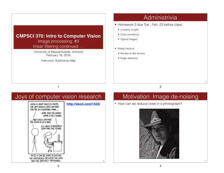
Administrivia Homework 2 due Tue., Feb. 23 before class Linearity - PowerPoint PPT Presentation
Administrivia Homework 2 due Tue., Feb. 23 before class Linearity of light Color constancy CMPSCI 370: Intro to Computer Vision Hybrid images Image processing: #3 linear filtering continued Todays lecture
Administrivia • Homework 2 due Tue., Feb. 23 before class • Linearity of light • Color constancy CMPSCI 370: Intro to Computer Vision • Hybrid images Image processing: #3 linear filtering continued … • Today’s lecture University of Massachusetts, Amherst • Review of last lecture February 18, 2016 • Edge detection Instructor: Subhransu Maji 2 1 2 Joys of computer vision research Motivation: Image de-noising • How can we reduce noise in a photograph? http://xkcd.com/1425/ 3 4 3 4
Moving average Convolution • Let’s replace each pixel with a weighted average of its • Let f be the image and g be the kernel. The output of convolving f with g is denoted f * g . neighborhood • The weights are called the filter kernel ( f g )[ m , n ] f [ m k , n l ] g [ k , l ] ∑ ∗ = − − • What are the weights for the average of a 3x3 k , l neighborhood? 1 1 1 f Convention: 1 1 1 kernel is “flipped” for convolution 1 1 1 “box filter” • MATLAB functions: conv2, filter2, imfilter Source: D. Lowe Source: F. Durand 5 6 5 6 Gaussian vs. box filtering Reducing salt-and-pepper noise 3x3 5x5 7x7 Gaussian smoothing fails to get rid of salt-and-pepper noise 7 8 7 8
Alternative idea: Median filtering Median filter • A median filter operates over a window by selecting the • What advantage does median filtering have over Gaussian median intensity in the window filtering? • Answer: Robustness to outliers The median filtering is not linear Source: K. Grauman Source: K. Grauman 9 10 9 10 Median filter Gaussian vs. median filtering 3x3 5x5 7x7 Median filtered Salt-and-pepper noise Gaussian Median MATLAB: medfilt2(image, [h w]) Source: M. Hebert 11 12 11 12
Sharpening revisited Sharpening filter I = blurry ( I ) + sharp ( I ) sharp ( I ) = I − blurry ( I ) What does blurring take away? = I ∗ e − I ∗ g σ = I ∗ ( e − g σ ) – = detail original smoothed (5x5) Let’s add it back: + α = unit impulse Gaussian Laplacian of Gaussian original detail sharpened 13 14 13 14 Application: Hybrid Images Gaussian Filter Laplacian Filter A. Oliva, A. Torralba, P.G. Schyns, “Hybrid Images,” SIGGRAPH 2006 15 15 16
motorcycle and bicycle dolphin and car 17 18 17 18 Homework 2, part 3 Next: edge detection Winter in Kraków photographed by Marcin Ryczek But first, any questions? 19 20 19 20
Edge detection Origin of edges • Goal: Identify sudden changes Edges are caused by a variety of factors: (discontinuities) in an image • Intuitively, most semantic and shape information from the image can be encoded in the edges surface normal discontinuity • More compact than pixels depth discontinuity • Ideal: artist’s line drawing (but artist is also using object-level surface color discontinuity knowledge) illumination discontinuity Attneave's Cat (1954) Source: D. Lowe 21 Source: Steve Seitz 22 21 22 Edge detection One dimensional derivatives • An edge is a place of rapid change in the image intensity m = ∆ y y = f ( x ) function Gradient ∆ x m = f ( x + h ) − f ( x ) = f ( x + h ) − f ( x ) intensity function image (along horizontal scanline) first derivative ( x + h ) − x h edges correspond to extrema of derivative https://en.wikipedia.org/wiki/Derivative 23 24 23 24
Two dimensional derivatives Partial derivatives with convolutions For 2D function f( x ), one can compute a derivative for each For 2D function f(x,y), the partial derivative is: direction v f ( x , y ) f ( x , y ) f ( x , y ) ∂ + ε − lim = x ∂ 0 ε ε → For discrete data, we can approximate using finite differences: f ( x , y ) f ( x 1 , y ) f ( x , y ) ∂ + − ≈ Directional derivatives of the function along the axes are called x 1 ∂ partial derivatives. For example the partial derivative with respect to x is: To implement the above as convolution, what would be f ( x , y ) f ( x , y ) f ( x , y ) ∂ + ε − the associated filter? lim = x ∂ 0 ε ε → Source: K. Grauman Source: K. Grauman 25 26 25 26 Finite difference filters Partial derivatives of an image Other approximations of derivative filters exist: f ( x , y ) f ( x , y ) ∂ ∂ x y ∂ ∂ -1 1 -1 1 or 1 -1 Which one shows changes with respect to x? Source: K. Grauman 27 28 27 28
Image gradient Edge detection example The gradient of an image: The gradient points in the direction of most rapid increase in intensity • How does this direction relate to the direction of the edge? image edge magnitude The gradient direction is given by The edge strength is given by the gradient magnitude Source: Steve Seitz https://en.wikipedia.org/wiki/Prewitt_operator 29 30 29 30 Edge detection in Matlab Effects of noise Consider a single row or column of the image Where is the edge? Source: S. Seitz 31 32 31 32
Solution: smooth first Scale of smoothing f g f * g 1 pixel 3 pixels 7 pixels d ( f g ) ∗ dx Smoothed derivative removes noise, but blurs edge. Also finds edges at different “scales” d • To find edges, look for peaks in ( f g ) ∗ dx Source: S. Seitz Source: D. Forsyth 33 34 33 34 Smoothing vs derivative filters Smoothing filters • Gaussian: remove “high-frequency” components; “low-pass” filter • Can the values of a smoothing filter be negative? • What should the values sum to? One: constant regions are not affected by the filter - Derivative filters • Prewitt filter • Can the values of a derivative filter be negative? • What should the values sum to? Zero: no response in constant regions - • High absolute value at points of high contrast 35 35
Recommend
More recommend
Explore More Topics
Stay informed with curated content and fresh updates.
