Administrivia Clear (10); mostly clear (7); unclear (6). Lecture 5 - PowerPoint PPT Presentation
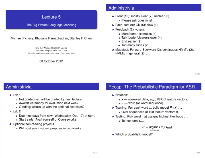
Administrivia Clear (10); mostly clear (7); unclear (6). Lecture 5 Please ask questions! Pace: fast (9); OK (6); slow (1). The Big Picture/Language Modeling Feedback (2+ votes): More/better examples (4). Talk louder/clearer/slower (4).
Administrivia Clear (10); mostly clear (7); unclear (6). Lecture 5 Please ask questions! Pace: fast (9); OK (6); slow (1). The Big Picture/Language Modeling Feedback (2+ votes): More/better examples (4). Talk louder/clearer/slower (4). Michael Picheny, Bhuvana Ramabhadran, Stanley F. Chen End earlier (2). Too many slides (2). IBM T.J. Watson Research Center Muddiest: Forward-Backward (3); continuous HMM’s (2); Yorktown Heights, New York, USA {picheny,bhuvana,stanchen}@us.ibm.com HMM’s in general (2); . . . 08 October 2012 2 / 121 Administrivia Recap: The Probabilistic Paradigm for ASR Lab 1 Notation: Not graded yet; will be graded by next lecture. x — observed data, e.g. , MFCC feature vectors. Awards ceremony for evaluation next week. ω — word (or word sequence). Grading: what’s up with the optional exercises? Training: For each word ω , build model P ω ( x ) . . . Lab 2 Over sequences of 40d feature vectors x . Due nine days from now (Wednesday, Oct. 17) at 6pm. Testing: Pick word that assigns highest likelihood . . . Start early! Avail yourself of Courseworks. To test data x test . Optional non-reading projects. ω ∗ = arg max P ω ( x test ) Will post soon; submit proposal in two weeks. ω ∈ vocab Which probabilistic model? 3 / 121 4 / 121
Part I Where Are We? Review 1 The HMM/GMM Framework Technical Details 2 Continuous Word Recognition 3 Discussion 4 5 / 121 6 / 121 The Basic Idea What is an HMM? Use separate HMM to model each word. Has states S and arcs/transitions a . Word is composed of sequence of “sounds”. Has start state S 0 (or start distribution). e.g. , BIT is composed of sounds “ B ”, “ IH ”, “ T ”. Has transition probabilities p a . Use HMM to model which sounds follow each other. Has output probabilities P ( � x | a ) on arcs (or states). e.g. , first, expect features for “ B ” sound, . . . Discrete: multinomial or single output. Then features for “ IH ” sound, etc. Continuous: GMM or other. For each sound, use GMM’s to model likely feature vectors. e.g. , what feature vectors are likely for “ B ” sound. ❣ ✶ ✴✵✳✺ ❣ ✷ ✴✵✳✺ ❣ ✸ ✴✵✳✺ ❣ ✹ ✴✵✳✺ ❣ ✺ ✴✵✳✺ ❣ ✻ ✴✵✳✺ ❣ ✶ ✴✵✳✺ ❣ ✷ ✴✵✳✺ ❣ ✸ ✴✵✳✺ ❣ ✹ ✴✵✳✺ ❣ ✺ ✴✵✳✺ ❣ ✻ ✴✵✳✺ 7 / 121 8 / 121
What Does an HMM Do? HMM’s and ASR Assigns probabilities P ( x ) to observation sequences: One HMM per word. A standard topology. x = � x 1 , . . . ,� x T ❣ ✶ ✴✵✳✺ ❣ ✷ ✴✵✳✺ ❣ ✸ ✴✵✳✺ ❣ ✹ ✴✵✳✺ ❣ ✺ ✴✵✳✺ ❣ ✻ ✴✵✳✺ ❣ ✶ ✴✵✳✺ ❣ ✷ ✴✵✳✺ ❣ ✸ ✴✵✳✺ ❣ ✹ ✴✵✳✺ ❣ ✺ ✴✵✳✺ ❣ ✻ ✴✵✳✺ Each x can be output by many paths through HMM. Path consists of sequence of arcs A = a 1 , . . . , a T . Use diagonal covariance GMM’s for output distributions. Compute P ( x ) by summing over path likelihoods. � � P ( � x | a ) = p a , j N ( x d ; µ a , j , d , σ a , j , d ) � P ( x ) = P ( x , A ) comp j dim d paths A Compute path likelihood by . . . Multiplying transition and output probs along path. T � p a t × P ( � P ( x , A ) = x t | a t ) t = 1 9 / 121 10 / 121 The Full Model The Viterbi and Forward Algorithms The Forward algorithm. � P ( x ) = P ( x , A ) � P ( x ) = P ( x , A ) paths A T paths A � � = p a t × P ( � x t | a t ) The Viterbi algorithm. paths A t = 1 T bestpath ( x ) = arg max P ( x , A ) � � � � N ( x t , d ; µ a t , j , d , σ 2 = p a t p a t , j a t , j , d ) paths A paths A t = 1 comp j dim d Can handle exponential number of paths A . . . p a — transition probability for arc a . In time linear in number of states, number of frames. ∗ p a , j — mixture weight, j th component of GMM on arc a . µ a , j , d — mean, d th dim, j th component, GMM on arc a . σ 2 a , j , d — variance, d th dim, j th component, GMM on arc a . ∗ Assuming fixed number of arcs per state. 11 / 121 12 / 121
Decoding The Forward-Backward Algorithm For each HMM, train parameters ( p a , p a , j , µ a , j , d , σ 2 Given trained HMM for each word ω . a , j , d ) . . . Use Forward algorithm to compute P ω ( x test ) for each ω . Using instances of that word in training set. Given initial parameter values, . . . Pick word that assigns highest likelihood. Iteratively finds local optimum in likelihood. ω ∗ = arg max P ω ( x test ) Dynamic programming version of EM algorithm. ω ∈ vocab Each iteration linear in number of states, number of frames. May need to do up to tens of iterations. 13 / 121 14 / 121 Example: Speech Data Training First two dimensions using Lab 1 front end; the word TWO . ❣ ✶ ✴✵✳✺ ❣ ✷ ✴✵✳✺ ❣ ✸ ✴✵✳✺ ❣ ✹ ✴✵✳✺ ❣ ✺ ✴✵✳✺ ❣ ✻ ✴✵✳✺ ❣ ✶ ✴✵✳✺ ❣ ✷ ✴✵✳✺ ❣ ✸ ✴✵✳✺ ❣ ✹ ✴✵✳✺ ❣ ✺ ✴✵✳✺ ❣ ✻ ✴✵✳✺ 15 / 121 16 / 121
The Viterbi Path Recap HMM/GMM framework can model arbitrary distributions . . . Over sequences of continuous vectors. Can train and decode efficiently. Forward, Viterbi, Forward-Backward algorithms. 17 / 121 18 / 121 Where Are We? The Smallest Number in the World Demo. Review 1 Technical Details 2 Continuous Word Recognition 3 Discussion 4 19 / 121 20 / 121
Probabilities and Log Probabilities Viterbi Algorithm and Max is Easy T � � � � N ( x t , d ; µ a t , j , d , σ 2 P ( x ) = p a t p a t , j a t , j , d ) x t P ( S ′ α ( S ′ , t − 1 ) α ( S , t ) = max ˆ → S ) × ˆ S ′ xt paths A t = 1 comp j dim d → S � � x t log P ( S ′ → S ) + log ˆ α ( S ′ , t − 1 ) log ˆ α ( S , t ) = max 1 sec of data ⇒ T = 100 ⇒ Multiply 4,000 likelihoods. S ′ xt → S Easy to generate values below 10 − 307 . Cannot store in C/C++ 64-bit double. Solution: store log probs instead of probs. e.g. , in Forward algorithm, instead of storing α ( S , t ) , . . . Store values log α ( S , t ) 21 / 121 22 / 121 Forward Algorithm and Sum is Tricky Decisions, Decisions . . . x t � P ( S ′ → S ) × α ( S ′ , t − 1 ) α ( S , t ) = HMM topology. S ′ xt Size of HMM’s. → S Size of GMM’s. � � x t � log P ( S ′ → S ) + log α ( S ′ , t − 1 ) Initial parameter values. log α ( S , t ) = log exp S ′ xt That’s it!? → S � � x t � × e C = log exp log P ( S ′ → S ) + log α ( S ′ , t − 1 ) − C S ′ xt → S � x t � � = C + log log P ( S ′ → S ) + log α ( S ′ , t − 1 ) − C exp S ′ xt → S How to pick C ? See Holmes, p. 153–154. 23 / 121 24 / 121
Which HMM Topology? How Many States? A standard topology. Rule of thumb: three states per phoneme. Must say sounds of word in order. Example: TWO is composed of phonemes T UW . Can stay at each sound indefinitely. Two phonemes ⇒ six HMM states. Different output distribution for each sound. ❣ ✹ ✴✵✳✺ ❣ ✺ ✴✵✳✺ ❣ ✻ ✴✵✳✺ ❣ ✶ ✴✵✳✺ ❣ ✷ ✴✵✳✺ ❣ ✸ ✴✵✳✺ ❣ ✶ ✴✵✳✺ ❣ ✷ ✴✵✳✺ ❣ ✸ ✴✵✳✺ ❣ ✹ ✴✵✳✺ ❣ ✺ ✴✵✳✺ ❣ ✻ ✴✵✳✺ ❣ ✶ ✴✵✳✺ ❣ ✷ ✴✵✳✺ ❣ ✸ ✴✵✳✺ ❣ ✹ ✴✵✳✺ ❣ ✺ ✴✵✳✺ ❣ ✻ ✴✵✳✺ ❚ ✶ ❚ ✷ ❚ ✸ ❯❲ ✶ ❯❲ ✷ ❯❲ ✸ ❣ ✶ ✴✵✳✺ ❣ ✷ ✴✵✳✺ ❣ ✸ ✴✵✳✺ ❣ ✹ ✴✵✳✺ ❣ ✺ ✴✵✳✺ ❣ ✻ ✴✵✳✺ No guarantee which sound each state models. Can we skip sounds, e.g. , fifth ? States are hidden! Use skip arcs ⇔ arcs with no output. Need to modify Forward, Viterbi, etc. ❣ ✶ ✴✵✳✹ ❣ ✷ ✴✵✳✹ ❣ ✸ ✴✵✳✹ ❣ ✹ ✴✵✳✹ ❣ ✺ ✴✵✳✹ ❣ ✻ ✴✵✳✹ ❣ ✶ ✴✵✳✹ ❣ ✷ ✴✵✳✹ ❣ ✸ ✴✵✳✹ ❣ ✹ ✴✵✳✹ ❣ ✺ ✴✵✳✹ ❣ ✻ ✴✵✳✹ ✎ ✴✵✳✷ ✎ ✴✵✳✷ ✎ ✴✵✳✷ ✎ ✴✵✳✷ ✎ ✴✵✳✷ 25 / 121 26 / 121 How Many GMM Components? Initial Parameter Values: Flat Start Use theory, e.g. , Bayesian Information Criterion (lecture 3). Transition probabilites p a — uniform. Just try different values. Mixture weights p a , j — uniform. Maybe 20–40, depending on how much data you have. Means µ a , j , d — 0. Variances σ 2 Empirical performance trumps theory any day of week. a , j , d — 1. Start with single component GMM. Run FB; split each Gaussian every few iters . . . Until reach target number of components per GMM. This actually works! (More on this in future lecture.) 27 / 121 28 / 121
Recommend
More recommend
Explore More Topics
Stay informed with curated content and fresh updates.
