Adaptive/Self-Tuning PID Control by Frequency Loop-Shaping Elena - PowerPoint PPT Presentation
Adaptive/Self-Tuning PID Control by Frequency Loop-Shaping Elena Grassi, ASU Kostas Tsakalis, ASU Sachi Dash, Honeywell HTC Sujit Gaikwad, Honeywell HTC Gunter Stein, Honeywell HTC CDC 00, Sydney 1 Outline Problem Description: PID
Adaptive/Self-Tuning PID Control by Frequency Loop-Shaping Elena Grassi, ASU Kostas Tsakalis, ASU Sachi Dash, Honeywell HTC Sujit Gaikwad, Honeywell HTC Gunter Stein, Honeywell HTC CDC 00, Sydney 1
Outline • Problem Description: PID Tuning from Input-Output data • Frequency Loop Shaping – Off-line tuning – Target loop selection, 1st-2nd order targets • Direct Adaptation of the PID parameters – Cost functional – Regressor generation via filter banks – Adaptation – Performance Monitoring Implications • Simulation Results • Conclusions CDC 00, Sydney 2
Problem Description • Industrial Applications – Large number of PID loops, often poorly tuned – Reliability and expediency requirements • A Variety of PID Tuning Strategies – Complete or partial models. (System identification-based vs. crossover properties) – Control objectives (Time-Frequency domain) – Direct and indirect approaches to adaptation • Frequency Loop Shaping – Accounting for uncertainty, several successful applications CDC 00, Sydney 3
FLS PID Tuning (batch/off-line) • System ID-modeling from I/O data • Nominal model & uncertainty bounds • Control Objective – Loop-shaping (sensitivity targets) – Disturbance attenuation subject to bandwidth constraints – Guide: “Robust Stability Condition” • On-line version via indirect adaptation – Update plant model, re-tune controller – Complete solutions can be computationally demanding – Simple models => off-line construction of look-up table for the PID gains CDC 00, Sydney 4
Target Loop Selection and FLS PID Tuning ( s a ) ( s a ) λ λ + λ + • Typical Targets: , , , ! 2 s s s ( s ) + ε – Target order depends open-loop/closed-loop bandwidth ratio (for input disturbance attenuation) – Uncertainty constraints and RHP pole-zero limitations – More difficult cases via LQ or full-order controller design methods e.g., K=lqr(A,B,Q,R), target: [A,B,K,0] • FLS Tuning: convex optimization in the frequency domain min S ( GC ( ) L ) min S ( GC ( ) L ) θ − θ − pid pid θ θ L pid L pid 2 ∞ s . t . constr . θ s . t . S ( GC ( ) L ) b θ − ≤ pid pid L ∞ constr . θ pid – L=loop gain, S=sensitivity, T=complementary sensitivity CDC 00, Sydney 5
Direct Adaptation with an FLS objective • Construction of the estimation error (at the plant input) e S ( CG L )[ u ] SC [ y ] T [ u ] = − = − e || || e ( ) sup S CG L e 2 − = L || u || ∞ u 0 ≠ 2 • Approximate sup by using a filter bank || SCF [ y ] TF [ u ] || || SCF [ y ] TF [ u ] || − − 2 , i i 2 δ S ( CG L ) max i i max − ≅ ≤ i i L || F [ u ] || || F [ u ] || ∞ i 2 i 2 , δ – F i : band-pass filters, ||.|| 2, δ : exponentially weighted 2-norm CDC 00, Sydney 6
Direct Adaptation with an FLS objective (cont.) J ( ) θ • Optimization problem i , k min max m M i θ ∈ i , k k ∑ k n T 2 J ( ) − | z w | θ = λ − θ i , k k i , n i , n k n 0 = 2 m m | F [ u ] | = λ + i , k i , k 1 i k − z TF [ u ] , w SC F [ y ] = = i , k i k i , k i k θ • Recursive computation of J i,k • Optimization: min-max of quadratics CDC 00, Sydney 7
Direct Adaptation details • Recursive computation of J i,k ˆ T T ( ) ( ) ( ) ( ) J J S 1 P θ = − θ − θ + θ − θ θ − θ i , k 1 i , k 1 i , k 1 k k i , k 1 k 2 + + + + ˆ T 2 J J ( ) | z w | = λ θ + − θ , 1 , , 1 , 1 i k i k k i k i k k + + + T T 2 , , 2 P P w w S R P R R z w = λ + = − θ = λ + i , k 1 i , k i , k i , k i , k 1 i , k 1 i , k 1 k i , k 1 i , k i , k i , k + + + + + • Each J i,k+1 is quadratic in the parameters: minimize the maximum by, e.g., computing a descent direction and performing a line search CDC 00, Sydney 8
Adaptive FLS Properties • Excitation requirements • Effects of disturbances and unmodeled dynamics (SNR) • A dead-zone condition: update when T 1 2 S P − S 2 d m 0 − > i , k i , k i , k 0 k – Update when the error operator gain drops by at least d 0 • Input Saturation does not affect updates • Linearization offsets (estimation or high-pass filtering) • The cost functional provides a measure of tuning confidence – Feasibility of performance monitoring CDC 00, Sydney 9
Example • Simulation Results for the following plant and target loop: 1 1 G ( s ) , L ( s ) = = 3 ( s 1 ) s + • Square-wave reference input. – Excitation injected at the plant input for t<75. • PID gains converge approximately to the off-line tuning. • Cost functional has a maximum of 0.3 2 , same as the off-line fitting error. CDC 00, Sydney 10
Simulation Results • Left: Parameters, output, reference, excitation. • Right: Square-root of cost functional. CDC 00, Sydney 11
Conclusions • Direct adaptation of PID parameters with an FLS objective – FLS: Operator gain interpretation of fitting error • Recursive implementation for on-line tuning • Use of a filter bank to approximate the min-max objective • Quantitative measures of tuning confidence – Gain of the error system Future work: • On-line monitoring of performance • On-line adaptation of objective (target loop) based on the cost functional values CDC 00, Sydney 12
Recommend
More recommend
Explore More Topics
Stay informed with curated content and fresh updates.
