Adaptive Density Estimation for Generative Models Thomas - PowerPoint PPT Presentation

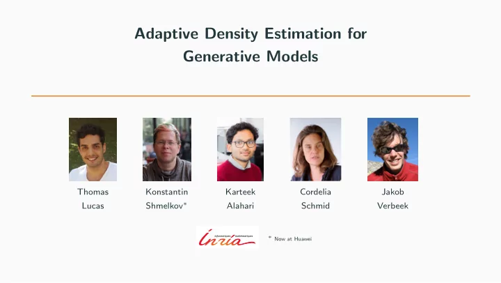
Adaptive Density Estimation for Generative Models Thomas Konstantin Karteek Cordelia Jakob Lucas Shmelkov ∗ Alahari Schmid Verbeek ∗ Now at Huawei

Generative modelling Goal Given samples from target distribution p ∗ , train a model p θ to match p ∗ 1

Generative modelling Goal Given samples from target distribution p ∗ , train a model p θ to match p ∗ • Maximum likelihood: Eval. training points under the model 1

Generative modelling Goal Given samples from target distribution p ∗ , train a model p θ to match p ∗ • Maximum likelihood: Eval. training points under the model • Adversarial training 1 : Eval. samples under (approximation of) p ∗ 1Ian Goodfellow et al. (2014). “Generative adversarial nets”. In: NIPS . 1

Schematic illustration Model Data 2

Maximum likelihood Model Data 3

Maximum likelihood Model Data Over-generalization 3

Maximum likelihood Consequences Model • MLE covers full support of distribution Data Over-generalization • Produces unrealistic samples 3

Adversarial training Mode-dropping 4

Adversarial training Consequences • Production of high quality samples • Parts of the support are dropped Mode-dropping 4

Hybrid training approach Goal • Explicitly optimize both dataset coverage and sample quality 5

Hybrid training approach Goal • Explicitly optimize both dataset coverage and sample quality • Discriminator can be seen as a learnable inductive bias 5

Hybrid training approach Goal • Explicitly optimize both dataset coverage and sample quality • Discriminator can be seen as a learnable inductive bias • Retain valid likelihood to evaluate support coverage 5

Hybrid training approach Goal • Explicitly optimize both dataset coverage and sample quality • Discriminator can be seen as a learnable inductive bias • Retain valid likelihood to evaluate support coverage Challenges • Tradeoff between the two objectives: need more flexibility 5

Hybrid training approach Goal • Explicitly optimize both dataset coverage and sample quality • Discriminator can be seen as a learnable inductive bias • Retain valid likelihood to evaluate support coverage Challenges • Tradeoff between the two objectives: need more flexibility • Limiting parametric assumptions required for tractable MLE, e.g. Gaussianity, conditional independence 5

Hybrid training approach Goal • Explicitly optimize both dataset coverage and sample quality • Discriminator can be seen as a learnable inductive bias • Retain valid likelihood to evaluate support coverage Challenges • Tradeoff between the two objectives: need more flexibility • Limiting parametric assumptions required for tractable MLE, e.g. Gaussianity, conditional independence • Often no likelihood in pixel space 2 2A. Larsen et al. (2016). “Autoencoding beyond pixels using a learned similarity metric”. In: ICML . 5

Conditional independence Data 6

Conditional independence N � p ( x | z ) = N ( x i | µ θ ( z ) , σ I n ) i Data 6

Conditional independence Strongly penalysed N by GAN � p ( x | z ) = N ( x i | µ θ ( z ) , σ I n ) Strongly i penalysed by MLE Data 6

Going beyond conditional independence Avoiding strong parametric assumptions • Lift reconstruction losses into a feature space 7

Going beyond conditional independence Avoiding strong parametric assumptions • Lift reconstruction losses into a feature space • Deep invertible models: valid density in image space 7

Going beyond conditional independence Avoiding strong parametric assumptions • Lift reconstruction losses into a feature space • Deep invertible models: valid density in image space • Retain fast sampling for adversarial training 7

Maximum likelihood estimation with feature targets 8

Maximum likelihood estimation with feature targets Amortized Variational inference in feature space : � � � det ∂f ψ � � L θ,φ,ψ ( x ) = − E q φ ( z | x ) [ln( p θ ( f ψ ( x ) | z ))] + D KL ( q φ ( z | x ) || p θ ( z )) − ln � � ∂ x � � �� � Evidence lower bound in feature space 8

Maximum likelihood estimation with feature targets Amortized Variational inference in feature space : � � � det ∂f ψ � � L θ,φ,ψ ( x ) = − E q φ ( z | x ) [ln( p θ ( f ψ ( x ) | z ))] + D KL ( q φ ( z | x ) || p θ ( z )) − ln � � ∂ x � � �� � Ch. of Var. 8

Maximum likelihood estimation with feature targets Maximum Likelihood Amortized Variational inference in feature space : � � � det ∂f ψ � � L θ,φ,ψ ( x ) = − E q φ ( z | x ) [ln( p θ ( f ψ ( x ) | z ))] + D KL ( q φ ( z | x ) || p θ ( z )) − ln � � ∂ x � 8

Maximum likelihood estimation with feature targets Maximum Likelihood Adv. training Amortized Variational inference in feature space : � � � det ∂f ψ � � L θ,φ,ψ ( x ) = − E q φ ( z | x ) [ln( p θ ( f ψ ( x ) | z ))] + D KL ( q φ ( z | x ) || p θ ( z )) − ln � � ∂ x � Adversarial training with Adaptive Density Estimation : � � D ( f − 1 ψ ( µ θ ( z ))) L adv ( p θ,ψ ) = − E p θ ( z ) ln 1 − D ( f − 1 ψ ( µ θ ( z ))) � �� � Adv. update using log ratio loss 8

Experiments on CIFAR10 Samples Real images 9

Experiments on CIFAR10 Model BPD ↓ IS ↑ FID ↓ GAN WGAN-GP 7 . 9 SNGAN 7 . 4 29 . 3 SNGAN ( R,H ) 8 . 2 21 . 7 MLE 3 . 8 † 73 . 5 † VAE-IAF 3 . 1 4 . 5 † 56 . 8 † NVP 3 . 5 Hybrid Ours (v1) 3 . 8 8 . 2 17 . 2 Ours (v2) 3 . 5 6 . 9 28 . 9 FlowGan 4 . 2 3 . 9 Samples Real images 9

Samples and real images (LSUN churches, 64 × 64 ) Samples @ 4 . 3 BPD Real images Thank you for listening. Come see us at poster 71 :) 10