Adaptive covariance inflation in the EnKF by Gaussian scale - PowerPoint PPT Presentation
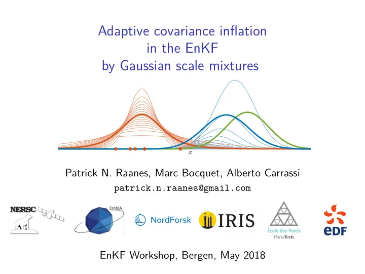
Adaptive covariance inflation in the EnKF by Gaussian scale mixtures pdf x Patrick N. Raanes, Marc Bocquet, Alberto Carrassi patrick.n.raanes@gmail.com NERSC NERSC EnKF Workshop, Bergen, May 2018 Questions answered in paper Nonlinear
Outline Idealistic contexts (with sampling error) Revisiting the EnKF assumptions = ⇒ Gaussian scale mixture (EnKF- N ) With model error Survey inflation estimation ETKF-adaptive EAKF-adaptive EnKF- N hybrid Benchmarks
Outline Idealistic contexts (with sampling error) Revisiting the EnKF assumptions = ⇒ Gaussian scale mixture (EnKF- N ) With model error Survey inflation estimation ETKF-adaptive EAKF-adaptive EnKF- N hybrid Benchmarks
Outline Idealistic contexts (with sampling error) Revisiting the EnKF assumptions = ⇒ Gaussian scale mixture (EnKF- N ) With model error Survey inflation estimation ETKF-adaptive EAKF-adaptive EnKF- N hybrid Benchmarks
Outline Idealistic contexts (with sampling error) Revisiting the EnKF assumptions = ⇒ Gaussian scale mixture (EnKF- N ) With model error Survey inflation estimation ETKF-adaptive EAKF-adaptive EnKF- N hybrid Benchmarks
Outline Idealistic contexts (with sampling error) Revisiting the EnKF assumptions = ⇒ Gaussian scale mixture (EnKF- N ) With model error Survey inflation estimation ETKF-adaptive EAKF-adaptive EnKF- N hybrid Benchmarks
Outline Idealistic contexts (with sampling error) Revisiting the EnKF assumptions = ⇒ Gaussian scale mixture (EnKF- N ) With model error Survey inflation estimation ETKF-adaptive EAKF-adaptive EnKF- N hybrid Benchmarks
Idealistic contexts (EnKF- N ) Assume M , H , Q , R are perfectly known, and p ( x ) and p ( y | x ) are always Gaussian.
EnKF
Revisiting EnKF assumptions Denote y prior all prior information on the “true” state, x ∈ R M , and suppose that, with known mean ( b ) and cov ( B ), p ( x | y prior ) = N ( x | b , B ) . (1) Computational costs induce: �� ≈ p ( x | E ) N ( x | b , B ) p ( b , B | E ) d b d B = ⇒ “true” moments, b and B , are unknowns, = to be estimated from E . � � Ensemble E = also from (1) and iid. x 1 , . . . x n , . . . x N
Revisiting EnKF assumptions Denote y prior all prior information on the “true” state, x ∈ R M , and suppose that, with known mean ( b ) and cov ( B ), p ( x | y prior ) = N ( x | b , B ) . (1) Computational costs induce: �� ≈ p ( x | E ) N ( x | b , B ) p ( b , B | E ) d b d B = ⇒ “true” moments, b and B , are unknowns, = to be estimated from E . � � Ensemble E = also from (1) and iid. x 1 , . . . x n , . . . x N
Revisiting EnKF assumptions Denote y prior all prior information on the “true” state, x ∈ R M , and suppose that, with known mean ( b ) and cov ( B ), p ( x | y prior ) = N ( x | b , B ) . (1) Computational costs induce: �� ≈ p ( x | E ) N ( x | b , B ) p ( b , B | E ) d b d B = ⇒ “true” moments, b and B , are unknowns, = to be estimated from E . � � Ensemble E = also from (1) and iid. x 1 , . . . x n , . . . x N
Revisiting EnKF assumptions Denote y prior all prior information on the “true” state, x ∈ R M , and suppose that, with known mean ( b ) and cov ( B ), p ( x | y prior ) = N ( x | b , B ) . (1) Computational costs induce: �� ≈ p ( x | E ) N ( x | b , B ) p ( b , B | E ) d b d B = ⇒ “true” moments, b and B , are unknowns, = to be estimated from E . � � Ensemble E = also from (1) and iid. x 1 , . . . x n , . . . x N
Revisiting EnKF assumptions Denote y prior all prior information on the “true” state, x ∈ R M , and suppose that, with known mean ( b ) and cov ( B ), p ( x | y prior ) = N ( x | b , B ) . (1) Computational costs induce: �� ≈ p ( x | E ) N ( x | b , B ) p ( b , B | E ) d b d B = ⇒ “true” moments, b and B , are unknowns, = to be estimated from E . � � Ensemble E = also from (1) and iid. x 1 , . . . x n , . . . x N
Revisiting EnKF assumptions Denote y prior all prior information on the “true” state, x ∈ R M , and suppose that, with known mean ( b ) and cov ( B ), p ( x | y prior ) = N ( x | b , B ) . (1) Computational costs induce: �� ≈ p ( x | E ) N ( x | b , B ) p ( b , B | E ) d b d B = ⇒ “true” moments, b and B , are unknowns, = to be estimated from E . � � Ensemble E = also from (1) and iid. x 1 , . . . x n , . . . x N
Revisiting EnKF assumptions Denote y prior all prior information on the “true” state, x ∈ R M , and suppose that, with known mean ( b ) and cov ( B ), p ( x | y prior ) = N ( x | b , B ) . (1) Computational costs induce: �� ≈ p ( x | E ) N ( x | b , B ) p ( b , B | E ) d b d B = ⇒ “true” moments, b and B , are unknowns, = to be estimated from E . � � Ensemble E = also from (1) and iid. x 1 , . . . x n , . . . x N
Revisiting EnKF assumptions Denote y prior all prior information on the “true” state, x ∈ R M , and suppose that, with known mean ( b ) and cov ( B ), p ( x | y prior ) = N ( x | b , B ) . (1) Computational costs induce: �� ≈ p ( x | E ) N ( x | b , B ) p ( b , B | E ) d b d B = ⇒ “true” moments, b and B , are unknowns, = to be estimated from E . � � Ensemble E = also from (1) and iid. x 1 , . . . x n , . . . x N
Revisiting EnKF assumptions Denote y prior all prior information on the “true” state, x ∈ R M , and suppose that, with known mean ( b ) and cov ( B ), p ( x | y prior ) = N ( x | b , B ) . (1) Computational costs induce: �� ≈ p ( x | E ) N ( x | b , B ) p ( b , B | E ) d b d B = ⇒ “true” moments, b and B , are unknowns, = to be estimated from E . � � Ensemble E = also from (1) and iid. x 1 , . . . x n , . . . x N
EnKF prior But � � p ( x | E ) = N ( x | b , B ) p ( b , B | E ) d b d B (2) B R M Recover standard EnKF by assuming N = ∞ so that x ) δ ( B − ¯ p ( b , B | E ) = δ ( b − ¯ B ) , where N N x = 1 1 � � x ) T . ¯ ( x n − ¯ x ) ( x n − ¯ ¯ x n , B = (3) N N − 1 n =1 n =1 The EnKF- N does not make this approximation.
EnKF prior But � � p ( x | E ) = N ( x | b , B ) p ( b , B | E ) d b d B (2) B R M Recover standard EnKF by assuming N = ∞ so that x ) δ ( B − ¯ p ( b , B | E ) = δ ( b − ¯ B ) , where N N x = 1 1 � � x ) T . ¯ ( x n − ¯ x ) ( x n − ¯ ¯ x n , B = (3) N N − 1 n =1 n =1 The EnKF- N does not make this approximation.
EnKF prior But � � p ( x | E ) = N ( x | b , B ) p ( b , B | E ) d b d B (2) B R M Recover standard EnKF by assuming N = ∞ so that x ) δ ( B − ¯ p ( b , B | E ) = δ ( b − ¯ B ) , where N N x = 1 1 � � x ) T . ¯ ( x n − ¯ x ) ( x n − ¯ ¯ x n , B = (3) N N − 1 n =1 n =1 The EnKF- N does not make this approximation.
EnKF- N via scale mixture �� Prior: p ( x | E ) = N ( x | b , B ) p ( b , B | E ) d b d B (4) (5) (6) (8)
EnKF- N via scale mixture �� Prior: p ( x | E ) = N ( x | b , B ) p ( b , B | E ) d b d B (4) . . . . . . (5) . . . . . . (6) . . . � − N/ 2 � x � 2 1 ∝ 1 + N − 1 � x − ¯ (7) ε N ¯ B (8)
EnKF- N via scale mixture �� Prior: p ( x | E ) = N ( x | b , B ) p ( b , B | E ) d b d B (4) . . . � � p � d α � � x − ¯ � α | E ∝ N x � ε N ¯ B | 0 , α α> 0 (5) . . . . . . (6) . . . � − N/ 2 � x � 2 1 ∝ 1 + N − 1 � x − ¯ (7) ε N ¯ B (8)
EnKF- N via scale mixture �� Prior: p ( x | E ) = N ( x | b , B ) p ( b , B | E ) d b d B (4) . . . � � p � d α � � x − ¯ � α | E ∝ N x � ε N ¯ B | 0 , α α> 0 (5) . . . . . . (6) . . . � − N/ 2 � x � 2 1 ∝ 1 + N − 1 � x − ¯ (7) ε N ¯ B � y | H x , R � p ( x | E , y ) ∝ p ( x | E ) N Posterior: (8)
EnKF- N via scale mixture �� Prior: p ( x | E ) = N ( x | b , B ) p ( b , B | E ) d b d B (4) . . . � � p � d α � � x − ¯ � α | E ∝ N x � ε N ¯ B | 0 , α α> 0 (5) . . . � ˜ � x | ¯ � α ( x ) | E � x , α ( x ) ¯ ∝ N p (6) B . . . � − N/ 2 � x � 2 1 ∝ 1 + N − 1 � x − ¯ (7) ε N ¯ B � y | H x , R � p ( x | E , y ) ∝ p ( x | E ) N Posterior: (8)
Mixing distributions – p ( α | . . . ) Prior pdf Posterior Likelihood 0 1 2 3 4 5 6 λ p ( α | E ) = χ − 2 ( α | 1 , N − 1) Prior: � − 1 x � 2 � Likelihood: p ( x ⋆ , y | α, E ) ∝ exp 2 � y − H¯ αε N H¯ BH T + R � − 1 � = ⇒ Posterior: p ( x ⋆ , α | y , E ) ∝ exp 2 D ( α )
Summary – Perfect model scenario Even with a perfect model, Gaussian forecasts, and a deterministic EnKF, “sampling error” arises for N < ∞ due to nonlinearity, and inflation is necessary. Not assuming ¯ B = B as in the EnKF leads to a Gaussian scale mixture. This leads to an adaptive inflation scheme, nullifying the need to tune the inflation factor, and yielding very strong benchmarks in idealistic settings. Excellent training for EnKF theory. Especially general-purpose inflation estimation.
Summary – Perfect model scenario Even with a perfect model, Gaussian forecasts, and a deterministic EnKF, “sampling error” arises for N < ∞ due to nonlinearity, and inflation is necessary. Not assuming ¯ B = B as in the EnKF leads to a Gaussian scale mixture. This leads to an adaptive inflation scheme, nullifying the need to tune the inflation factor, and yielding very strong benchmarks in idealistic settings. Excellent training for EnKF theory. Especially general-purpose inflation estimation.
Summary – Perfect model scenario Even with a perfect model, Gaussian forecasts, and a deterministic EnKF, “sampling error” arises for N < ∞ due to nonlinearity, and inflation is necessary. Not assuming ¯ B = B as in the EnKF leads to a Gaussian scale mixture. This leads to an adaptive inflation scheme, nullifying the need to tune the inflation factor, and yielding very strong benchmarks in idealistic settings. Excellent training for EnKF theory. Especially general-purpose inflation estimation.
Summary – Perfect model scenario Even with a perfect model, Gaussian forecasts, and a deterministic EnKF, “sampling error” arises for N < ∞ due to nonlinearity, and inflation is necessary. Not assuming ¯ B = B as in the EnKF leads to a Gaussian scale mixture. This leads to an adaptive inflation scheme, nullifying the need to tune the inflation factor, and yielding very strong benchmarks in idealistic settings. Excellent training for EnKF theory. Especially general-purpose inflation estimation.
Summary – Perfect model scenario Even with a perfect model, Gaussian forecasts, and a deterministic EnKF, “sampling error” arises for N < ∞ due to nonlinearity, and inflation is necessary. Not assuming ¯ B = B as in the EnKF leads to a Gaussian scale mixture. This leads to an adaptive inflation scheme, nullifying the need to tune the inflation factor, and yielding very strong benchmarks in idealistic settings. Excellent training for EnKF theory. Especially general-purpose inflation estimation.
Summary – Perfect model scenario Even with a perfect model, Gaussian forecasts, and a deterministic EnKF, “sampling error” arises for N < ∞ due to nonlinearity, and inflation is necessary. Not assuming ¯ B = B as in the EnKF leads to a Gaussian scale mixture. This leads to an adaptive inflation scheme, nullifying the need to tune the inflation factor, and yielding very strong benchmarks in idealistic settings. Excellent training for EnKF theory. Especially general-purpose inflation estimation.
With model error Because all models are wrong.
Fundamentals � b , B /β � , and N = ∞ . Suppose x n ∼ N Then there’s no mixture, but simply � . � � x x , β ¯ p ( x | β, ) = N (9) � ¯ B Recall � . � y | H x , R p ( y | x ) = N Then � y � � � H¯ x , ¯ p ( y | β ) = N C ( β ) , BH T + R , C ( β ) = β H¯ ¯ where (10)
Fundamentals � b , B /β � , and N = ∞ . Suppose x n ∼ N Then there’s no mixture, but simply � . � � x x , β ¯ p ( x | β, ) = N (9) � ¯ B Recall � . � y | H x , R p ( y | x ) = N Then � y � � � H¯ x , ¯ p ( y | β ) = N C ( β ) , BH T + R , C ( β ) = β H¯ ¯ where (10)
Fundamentals � b , B /β � , and N = ∞ . Suppose x n ∼ N Then there’s no mixture, but simply � . � � x x , β ¯ p ( x | β, ) = N (9) � ¯ B Recall � . � y | H x , R p ( y | x ) = N Then � y � � � H¯ x , ¯ p ( y | β ) = N C ( β ) , BH T + R , C ( β ) = β H¯ ¯ where (10)
Fundamentals � b , B /β � , and N = ∞ . Suppose x n ∼ N Then there’s no mixture, but simply � . � � x x , β ¯ p ( x | β, E ) = N (9) � ¯ B Recall � . � y | H x , R p ( y | x ) = N Then � y � � � H¯ x , ¯ p ( y | β ) = N C ( β ) , BH T + R , C ( β ) = β H¯ ¯ where (10)
Fundamentals � b , B /β � , and N = ∞ . Suppose x n ∼ N Then there’s no mixture, but simply � . � � x x , β ¯ p ( x | β, � � E ) = N (9) � ¯ B Recall � . � y | H x , R p ( y | x ) = N Then � y � � � H¯ x , ¯ p ( y | β ) = N C ( β ) , BH T + R , C ( β ) = β H¯ ¯ where (10)
Fundamentals � b , B /β � , and N = ∞ . Suppose x n ∼ N Then there’s no mixture, but simply � . � � x x , β ¯ p ( x | β, � � E ) = N (9) � ¯ B Recall � . � y | H x , R p ( y | x ) = N Then � y � � � H¯ x , ¯ p ( y | β ) = N C ( β ) , BH T + R , C ( β ) = β H¯ ¯ where (10)
Fundamentals � b , B /β � , and N = ∞ . Suppose x n ∼ N Then there’s no mixture, but simply � . � � x x , β ¯ p ( x | β, � � E ) = N (9) � ¯ B Recall � . � y | H x , R p ( y | x ) = N Then � y � � � H¯ x , ¯ p ( y | β ) = N C ( β ) , BH T + R , C ( β ) = β H¯ ¯ where (10)
Fundamentals � b , B /β � , and N = ∞ . Suppose x n ∼ N Then there’s no mixture, but simply � . � � x x , β ¯ p ( x | β, � � E ) = N (9) � ¯ B Recall � . � y | H x , R p ( y | x ) = N Then � = N � , � y � � ¯ � � H¯ x , ¯ � 0 , ¯ p ( y | β ) = N C ( β ) δ C ( β ) BH T + R , C ( β ) = β H¯ ¯ where ¯ δ = y − H¯ x . (10)
ETKF adaptive inflation Again, � , � � ¯ � 0 , ¯ p ( y | β ) = N C ( β ) (11) δ BH T + R ≈ ¯ δ T . C ( β ) = β H¯ ¯ δ ¯ where (12) “yielding” (Wang and Bishop, 2003) β R = � ¯ δ � 2 R /P − 1 ˆ , σ 2 ¯ σ 2 = tr( H¯ BH T R − 1 ) /P . where P = length ( y ) and ¯ Also considered: ˆ β I , ˆ BH T , ˆ β H¯ β ¯ C (1) , ML, VB (EM).
ETKF adaptive inflation Again, � , � � ¯ � 0 , ¯ p ( y | β ) = N C ( β ) (11) δ BH T + R ≈ ¯ δ T . C ( β ) = β H¯ ¯ δ ¯ where (12) “yielding” (Wang and Bishop, 2003) β R = � ¯ δ � 2 R /P − 1 ˆ , σ 2 ¯ σ 2 = tr( H¯ BH T R − 1 ) /P . where P = length ( y ) and ¯ Also considered: ˆ β I , ˆ BH T , ˆ β H¯ β ¯ C (1) , ML, VB (EM).
ETKF adaptive inflation Again, � , � � ¯ � 0 , ¯ p ( y | β ) = N C ( β ) (11) δ BH T + R ≈ ¯ δ T . C ( β ) = β H¯ ¯ δ ¯ where (12) “yielding” (Wang and Bishop, 2003) β R = � ¯ δ � 2 R /P − 1 ˆ , σ 2 ¯ σ 2 = tr( H¯ BH T R − 1 ) /P . where P = length ( y ) and ¯ Also considered: ˆ β I , ˆ BH T , ˆ β H¯ β ¯ C (1) , ML, VB (EM).
ETKF adaptive inflation Again, � , � � ¯ � 0 , ¯ p ( y | β ) = N C ( β ) (11) δ BH T + R ≈ ¯ δ T . C ( β ) = β H¯ ¯ δ ¯ where (12) “yielding” (Wang and Bishop, 2003) β R = � ¯ δ � 2 R /P − 1 ˆ , σ 2 ¯ σ 2 = tr( H¯ BH T R − 1 ) /P . where P = length ( y ) and ¯ Also considered: ˆ β I , ˆ BH T , ˆ β H¯ β ¯ C (1) , ML, VB (EM).
ETKF adaptive inflation Again, � , � � ¯ � 0 , ¯ p ( y | β ) = N C ( β ) (11) δ BH T + R ≈ ¯ δ T . C ( β ) = β H¯ ¯ δ ¯ where (12) “yielding” (Wang and Bishop, 2003) β R = � ¯ δ � 2 R /P − 1 ˆ , σ 2 ¯ σ 2 = tr( H¯ BH T R − 1 ) /P . where P = length ( y ) and ¯ Also considered: ˆ β I , ˆ BH T , ˆ β H¯ β ¯ C (1) , ML, VB (EM).
ETKF adaptive inflation Again, � , � � ¯ � 0 , ¯ p ( y | β ) = N C ( β ) (11) δ BH T + R ≈ ¯ δ T . C ( β ) = β H¯ ¯ δ ¯ where (12) “yielding” (Wang and Bishop, 2003) β R = � ¯ δ � 2 R /P − 1 ˆ , σ 2 ¯ σ 2 = tr( H¯ BH T R − 1 ) /P . where P = length ( y ) and ¯ Also considered: ˆ β I , ˆ BH T , ˆ β H¯ β ¯ C (1) , ML, VB (EM).
ETKF adaptive inflation Again, � , � � ¯ � 0 , ¯ p ( y | β ) = N C ( β ) (11) δ BH T + R ≈ ¯ δ T . C ( β ) = β H¯ ¯ δ ¯ where (12) “yielding” (Wang and Bishop, 2003) β R = � ¯ δ � 2 R /P − 1 ˆ , σ 2 ¯ σ 2 = tr( H¯ BH T R − 1 ) /P . where P = length ( y ) and ¯ Also considered: ˆ β I , ˆ BH T , ˆ β H¯ β ¯ C (1) , ML, VB (EM).
Renouncing Gaussianity BH T ∝ R . Assume H¯ � becomes � ¯ � � 0 , ¯ The likelihood p ( y | β ) = N δ C ( β ) : p ( y | β ) ∝ χ +2 � � � � ¯ δ � 2 σ 2 β ) , P � R /P � (1 + ¯ . (13) Surprise !!!: argmax p ( y | β ) = ˆ β R , A further approximation is fitted: p ( y | β ) ≈ χ +2 (ˆ β R | β, ˆ ν ) . (14) Likelihood (14) fits mode of (13). Fitting curvature = ⇒ ˆ ν = ⇒ same variance as in Miyoshi (2011) !!! Likelihood (14) conjugate to p ( β ) = χ − 2 ( β | β f , ν f ) , yielding ν a = ν f + ˆ ν , (15) β a = ( ν f β f + ˆ β R ) /ν a , ν ˆ (16) again, as in Miyoshi (2011).
Renouncing Gaussianity BH T ∝ R . Assume H¯ � becomes � ¯ � � 0 , ¯ The likelihood p ( y | β ) = N δ C ( β ) : p ( y | β ) ∝ χ +2 � � � � ¯ δ � 2 σ 2 β ) , P � R /P � (1 + ¯ . (13) Surprise !!!: argmax p ( y | β ) = ˆ β R , A further approximation is fitted: p ( y | β ) ≈ χ +2 (ˆ β R | β, ˆ ν ) . (14) Likelihood (14) fits mode of (13). Fitting curvature = ⇒ ˆ ν = ⇒ same variance as in Miyoshi (2011) !!! Likelihood (14) conjugate to p ( β ) = χ − 2 ( β | β f , ν f ) , yielding ν a = ν f + ˆ ν , (15) β a = ( ν f β f + ˆ β R ) /ν a , ν ˆ (16) again, as in Miyoshi (2011).
Renouncing Gaussianity BH T ∝ R . Assume H¯ � becomes � ¯ � � 0 , ¯ The likelihood p ( y | β ) = N δ C ( β ) : p ( y | β ) ∝ χ +2 � � � � ¯ δ � 2 σ 2 β ) , P � R /P � (1 + ¯ . (13) Surprise !!!: argmax p ( y | β ) = ˆ β R , A further approximation is fitted: p ( y | β ) ≈ χ +2 (ˆ β R | β, ˆ ν ) . (14) Likelihood (14) fits mode of (13). Fitting curvature = ⇒ ˆ ν = ⇒ same variance as in Miyoshi (2011) !!! Likelihood (14) conjugate to p ( β ) = χ − 2 ( β | β f , ν f ) , yielding ν a = ν f + ˆ ν , (15) β a = ( ν f β f + ˆ β R ) /ν a , ν ˆ (16) again, as in Miyoshi (2011).
Renouncing Gaussianity BH T ∝ R . Assume H¯ � becomes � ¯ � � 0 , ¯ The likelihood p ( y | β ) = N δ C ( β ) : p ( y | β ) ∝ χ +2 � � � � ¯ δ � 2 σ 2 β ) , P � R /P � (1 + ¯ . (13) Surprise !!!: argmax p ( y | β ) = ˆ β R , A further approximation is fitted: p ( y | β ) ≈ χ +2 (ˆ β R | β, ˆ ν ) . (14) Likelihood (14) fits mode of (13). Fitting curvature = ⇒ ˆ ν = ⇒ same variance as in Miyoshi (2011) !!! Likelihood (14) conjugate to p ( β ) = χ − 2 ( β | β f , ν f ) , yielding ν a = ν f + ˆ ν , (15) β a = ( ν f β f + ˆ β R ) /ν a , ν ˆ (16) again, as in Miyoshi (2011).
Renouncing Gaussianity BH T ∝ R . Assume H¯ � becomes � ¯ � � 0 , ¯ The likelihood p ( y | β ) = N δ C ( β ) : p ( y | β ) ∝ χ +2 � � � � ¯ δ � 2 σ 2 β ) , P � R /P � (1 + ¯ . (13) Surprise !!!: argmax p ( y | β ) = ˆ β R , A further approximation is fitted: p ( y | β ) ≈ χ +2 (ˆ β R | β, ˆ ν ) . (14) Likelihood (14) fits mode of (13). Fitting curvature = ⇒ ˆ ν = ⇒ same variance as in Miyoshi (2011) !!! Likelihood (14) conjugate to p ( β ) = χ − 2 ( β | β f , ν f ) , yielding ν a = ν f + ˆ ν , (15) β a = ( ν f β f + ˆ β R ) /ν a , ν ˆ (16) again, as in Miyoshi (2011).
Renouncing Gaussianity BH T ∝ R . Assume H¯ � becomes � ¯ � � 0 , ¯ The likelihood p ( y | β ) = N δ C ( β ) : p ( y | β ) ∝ χ +2 � � � � ¯ δ � 2 σ 2 β ) , P � R /P � (1 + ¯ . (13) Surprise !!!: argmax p ( y | β ) = ˆ β R , A further approximation is fitted: p ( y | β ) ≈ χ +2 (ˆ β R | β, ˆ ν ) . (14) Likelihood (14) fits mode of (13). Fitting curvature = ⇒ ˆ ν = ⇒ same variance as in Miyoshi (2011) !!! Likelihood (14) conjugate to p ( β ) = χ − 2 ( β | β f , ν f ) , yielding ν a = ν f + ˆ ν , (15) β a = ( ν f β f + ˆ β R ) /ν a , ν ˆ (16) again, as in Miyoshi (2011).
Renouncing Gaussianity BH T ∝ R . Assume H¯ � becomes � ¯ � � 0 , ¯ The likelihood p ( y | β ) = N δ C ( β ) : p ( y | β ) ∝ χ +2 � � � � ¯ δ � 2 σ 2 β ) , P � R /P � (1 + ¯ . (13) Surprise !!!: argmax p ( y | β ) = ˆ β R , A further approximation is fitted: p ( y | β ) ≈ χ +2 (ˆ β R | β, ˆ ν ) . (14) Likelihood (14) fits mode of (13). Fitting curvature = ⇒ ˆ ν = ⇒ same variance as in Miyoshi (2011) !!! Likelihood (14) conjugate to p ( β ) = χ − 2 ( β | β f , ν f ) , yielding ν a = ν f + ˆ ν , (15) β a = ( ν f β f + ˆ β R ) /ν a , ν ˆ (16) again, as in Miyoshi (2011).
Renouncing Gaussianity BH T ∝ R . Assume H¯ � becomes � ¯ � � 0 , ¯ The likelihood p ( y | β ) = N δ C ( β ) : p ( y | β ) ∝ χ +2 � � � � ¯ δ � 2 σ 2 β ) , P � R /P � (1 + ¯ . (13) Surprise !!!: argmax p ( y | β ) = ˆ β R , A further approximation is fitted: p ( y | β ) ≈ χ +2 (ˆ β R | β, ˆ ν ) . (14) Likelihood (14) fits mode of (13). Fitting curvature = ⇒ ˆ ν = ⇒ same variance as in Miyoshi (2011) !!! Likelihood (14) conjugate to p ( β ) = χ − 2 ( β | β f , ν f ) , yielding ν a = ν f + ˆ ν , (15) β a = ( ν f β f + ˆ β R ) /ν a , ν ˆ (16) again, as in Miyoshi (2011).
Renouncing Gaussianity BH T ∝ R . Assume H¯ � becomes � ¯ � � 0 , ¯ The likelihood p ( y | β ) = N δ C ( β ) : p ( y | β ) ∝ χ +2 � � � � ¯ δ � 2 σ 2 β ) , P � R /P � (1 + ¯ . (13) Surprise !!!: argmax p ( y | β ) = ˆ β R , A further approximation is fitted: p ( y | β ) ≈ χ +2 (ˆ β R | β, ˆ ν ) . (14) Likelihood (14) fits mode of (13). Fitting curvature = ⇒ ˆ ν = ⇒ same variance as in Miyoshi (2011) !!! Likelihood (14) conjugate to p ( β ) = χ − 2 ( β | β f , ν f ) , yielding ν a = ν f + ˆ ν , (15) β a = ( ν f β f + ˆ β R ) /ν a , ν ˆ (16) again, as in Miyoshi (2011).
Renouncing Gaussianity BH T ∝ R . Assume H¯ � becomes � ¯ � � 0 , ¯ The likelihood p ( y | β ) = N δ C ( β ) : p ( y | β ) ∝ χ +2 � � � � ¯ δ � 2 σ 2 β ) , P � R /P � (1 + ¯ . (13) Surprise !!!: argmax p ( y | β ) = ˆ β R , A further approximation is fitted: p ( y | β ) ≈ χ +2 (ˆ β R | β, ˆ ν ) . (14) Likelihood (14) fits mode of (13). Fitting curvature = ⇒ ˆ ν = ⇒ same variance as in Miyoshi (2011) !!! Likelihood (14) conjugate to p ( β ) = χ − 2 ( β | β f , ν f ) , yielding ν a = ν f + ˆ ν , (15) β a = ( ν f β f + ˆ β R ) /ν a , ν ˆ (16) again, as in Miyoshi (2011).
Renouncing Gaussianity BH T ∝ R . Assume H¯ � becomes � ¯ � � 0 , ¯ The likelihood p ( y | β ) = N δ C ( β ) : p ( y | β ) ∝ χ +2 � � � � ¯ δ � 2 σ 2 β ) , P � R /P � (1 + ¯ . (13) Surprise !!!: argmax p ( y | β ) = ˆ β R , A further approximation is fitted: p ( y | β ) ≈ χ +2 (ˆ β R | β, ˆ ν ) . (14) Likelihood (14) fits mode of (13). Fitting curvature = ⇒ ˆ ν = ⇒ same variance as in Miyoshi (2011) !!! Likelihood (14) conjugate to p ( β ) = χ − 2 ( β | β f , ν f ) , yielding ν a = ν f + ˆ ν , (15) β a = ( ν f β f + ˆ β R ) /ν a , ν ˆ (16) again, as in Miyoshi (2011).
EAKF adaptive inflation Anderson (2007) assigns Gaussian prior: p ( β ) = N ( β | β f , V f ) , (17) and fits the posterior by a “Gaussian”: p ( β | y i ) ≈ N ( β | ˆ β MAP , V a ) , (18) β MAP and V a are fitted using the exact posterior where ˆ (“easy” by virtue of serial update). Gharamti (2017) improves via χ − 2 and χ +2 (Gamma).
EAKF adaptive inflation Anderson (2007) assigns Gaussian prior: p ( β ) = N ( β | β f , V f ) , (17) and fits the posterior by a “Gaussian”: p ( β | y i ) ≈ N ( β | ˆ β MAP , V a ) , (18) β MAP and V a are fitted using the exact posterior where ˆ (“easy” by virtue of serial update). Gharamti (2017) improves via χ − 2 and χ +2 (Gamma).
EAKF adaptive inflation Anderson (2007) assigns Gaussian prior: p ( β ) = N ( β | β f , V f ) , (17) and fits the posterior by a “Gaussian”: p ( β | y i ) ≈ N ( β | ˆ β MAP , V a ) , (18) β MAP and V a are fitted using the exact posterior where ˆ (“easy” by virtue of serial update). Gharamti (2017) improves via χ − 2 and χ +2 (Gamma).
EAKF adaptive inflation Anderson (2007) assigns Gaussian prior: p ( β ) = N ( β | β f , V f ) , (17) and fits the posterior by a “Gaussian”: p ( β | y i ) ≈ N ( β | ˆ β MAP , V a ) , (18) β MAP and V a are fitted using the exact posterior where ˆ (“easy” by virtue of serial update). Gharamti (2017) improves via χ − 2 and χ +2 (Gamma).
EAKF adaptive inflation Anderson (2007) assigns Gaussian prior: p ( β ) = N ( β | β f , V f ) , (17) and fits the posterior by a “Gaussian”: p ( β | y i ) ≈ N ( β | ˆ β MAP , V a ) , (18) β MAP and V a are fitted using the exact posterior where ˆ (“easy” by virtue of serial update). Gharamti (2017) improves via χ − 2 and χ +2 (Gamma).
EnKF- N hybrid Use two inflation factors: α and β , dedicated to sampling and model error, respectively. For β , pick simplest (and ∼ best) scheme: ˆ β R . Algorithm: Find β (via ˆ β R ) Find α given β (via EnKF- N ) Potential improvements: Determining ( α, β ) jointly (simultaneously). Rather than fitting the likelihood parameters, fit posterior parameters (similarly to EAKF). Matching moments via quadrature Non-parametric (grid- or MC- based) De-biasing ˆ β R Testing “improvements” did not yield significant gains.
EnKF- N hybrid Use two inflation factors: α and β , dedicated to sampling and model error, respectively. For β , pick simplest (and ∼ best) scheme: ˆ β R . Algorithm: Find β (via ˆ β R ) Find α given β (via EnKF- N ) Potential improvements: Determining ( α, β ) jointly (simultaneously). Rather than fitting the likelihood parameters, fit posterior parameters (similarly to EAKF). Matching moments via quadrature Non-parametric (grid- or MC- based) De-biasing ˆ β R Testing “improvements” did not yield significant gains.
EnKF- N hybrid Use two inflation factors: α and β , dedicated to sampling and model error, respectively. For β , pick simplest (and ∼ best) scheme: ˆ β R . Algorithm: Find β (via ˆ β R ) Find α given β (via EnKF- N ) Potential improvements: Determining ( α, β ) jointly (simultaneously). Rather than fitting the likelihood parameters, fit posterior parameters (similarly to EAKF). Matching moments via quadrature Non-parametric (grid- or MC- based) De-biasing ˆ β R Testing “improvements” did not yield significant gains.
EnKF- N hybrid Use two inflation factors: α and β , dedicated to sampling and model error, respectively. For β , pick simplest (and ∼ best) scheme: ˆ β R . Algorithm: Find β (via ˆ β R ) Find α given β (via EnKF- N ) Potential improvements: Determining ( α, β ) jointly (simultaneously). Rather than fitting the likelihood parameters, fit posterior parameters (similarly to EAKF). Matching moments via quadrature Non-parametric (grid- or MC- based) De-biasing ˆ β R Testing “improvements” did not yield significant gains.
EnKF- N hybrid Use two inflation factors: α and β , dedicated to sampling and model error, respectively. For β , pick simplest (and ∼ best) scheme: ˆ β R . Algorithm: Find β (via ˆ β R ) Find α given β (via EnKF- N ) Potential improvements: Determining ( α, β ) jointly (simultaneously). Rather than fitting the likelihood parameters, fit posterior parameters (similarly to EAKF). Matching moments via quadrature Non-parametric (grid- or MC- based) De-biasing ˆ β R Testing “improvements” did not yield significant gains.
EnKF- N hybrid Use two inflation factors: α and β , dedicated to sampling and model error, respectively. For β , pick simplest (and ∼ best) scheme: ˆ β R . Algorithm: Find β (via ˆ β R ) Find α given β (via EnKF- N ) Potential improvements: Determining ( α, β ) jointly (simultaneously). Rather than fitting the likelihood parameters, fit posterior parameters (similarly to EAKF). Matching moments via quadrature Non-parametric (grid- or MC- based) De-biasing ˆ β R Testing “improvements” did not yield significant gains.
EnKF- N hybrid Use two inflation factors: α and β , dedicated to sampling and model error, respectively. For β , pick simplest (and ∼ best) scheme: ˆ β R . Algorithm: Find β (via ˆ β R ) Find α given β (via EnKF- N ) Potential improvements: Determining ( α, β ) jointly (simultaneously). Rather than fitting the likelihood parameters, fit posterior parameters (similarly to EAKF). Matching moments via quadrature Non-parametric (grid- or MC- based) De-biasing ˆ β R Testing “improvements” did not yield significant gains.
EnKF- N hybrid Use two inflation factors: α and β , dedicated to sampling and model error, respectively. For β , pick simplest (and ∼ best) scheme: ˆ β R . Algorithm: Find β (via ˆ β R ) Find α given β (via EnKF- N ) Potential improvements: Determining ( α, β ) jointly (simultaneously). Rather than fitting the likelihood parameters, fit posterior parameters (similarly to EAKF). Matching moments via quadrature Non-parametric (grid- or MC- based) De-biasing ˆ β R Testing “improvements” did not yield significant gains.
EnKF- N hybrid Use two inflation factors: α and β , dedicated to sampling and model error, respectively. For β , pick simplest (and ∼ best) scheme: ˆ β R . Algorithm: Find β (via ˆ β R ) Find α given β (via EnKF- N ) Potential improvements: Determining ( α, β ) jointly (simultaneously). Rather than fitting the likelihood parameters, fit posterior parameters (similarly to EAKF). Matching moments via quadrature Non-parametric (grid- or MC- based) De-biasing ˆ β R Testing “improvements” did not yield significant gains.
EnKF- N hybrid Use two inflation factors: α and β , dedicated to sampling and model error, respectively. For β , pick simplest (and ∼ best) scheme: ˆ β R . Algorithm: Find β (via ˆ β R ) Find α given β (via EnKF- N ) Potential improvements: Determining ( α, β ) jointly (simultaneously). Rather than fitting the likelihood parameters, fit posterior parameters (similarly to EAKF). Matching moments via quadrature Non-parametric (grid- or MC- based) De-biasing ˆ β R Testing “improvements” did not yield significant gains.
EnKF- N hybrid Use two inflation factors: α and β , dedicated to sampling and model error, respectively. For β , pick simplest (and ∼ best) scheme: ˆ β R . Algorithm: Find β (via ˆ β R ) Find α given β (via EnKF- N ) Potential improvements: Determining ( α, β ) jointly (simultaneously). Rather than fitting the likelihood parameters, fit posterior parameters (similarly to EAKF). Matching moments via quadrature Non-parametric (grid- or MC- based) De-biasing ˆ β R Testing “improvements” did not yield significant gains.
EnKF- N hybrid Use two inflation factors: α and β , dedicated to sampling and model error, respectively. For β , pick simplest (and ∼ best) scheme: ˆ β R . Algorithm: Find β (via ˆ β R ) Find α given β (via EnKF- N ) Potential improvements: Determining ( α, β ) jointly (simultaneously). Rather than fitting the likelihood parameters, fit posterior parameters (similarly to EAKF). Matching moments via quadrature Non-parametric (grid- or MC- based) De-biasing ˆ β R Testing “improvements” did not yield significant gains.
EnKF- N hybrid Use two inflation factors: α and β , dedicated to sampling and model error, respectively. For β , pick simplest (and ∼ best) scheme: ˆ β R . Algorithm: Find β (via ˆ β R ) Find α given β (via EnKF- N ) Potential improvements: Determining ( α, β ) jointly (simultaneously). Rather than fitting the likelihood parameters, fit posterior parameters (similarly to EAKF). Matching moments via quadrature Non-parametric (grid- or MC- based) De-biasing ˆ β R Testing “improvements” did not yield significant gains.
Two-layer Lorenz-96 Evolution 10 d x i + F − hc � ψ + d t = i ( x ) z j +10( i − 1) , i = 1 , . . . , 36 , b j =1 d z j d t = c j ( b z ) + 0 + hc bψ − bx 1+( j − 1) / / 10 , j = 1 , . . . , 360 , where ψ i is the single-layer Lorenz-96 dynamics. 10 Example snapshots 8 6 � 1 T 4 RMSE = 1 � x t − x t � 2 M � ¯ 2 . T 2 t =1 0 N = 20 , no localization. −2 −4 1 4 8 12 16 20 24 28 32 36 1 40 80 120 160 200 240 280 320 360
Two-layer Lorenz-96 Evolution 10 d x i + F − hc � ψ + d t = i ( x ) z j +10( i − 1) , i = 1 , . . . , 36 , b j =1 d z j d t = c j ( b z ) + 0 + hc bψ − bx 1+( j − 1) / / 10 , j = 1 , . . . , 360 , where ψ i is the single-layer Lorenz-96 dynamics. 10 Example snapshots 8 6 � 1 T 4 RMSE = 1 � x t − x t � 2 M � ¯ 2 . T 2 t =1 0 N = 20 , no localization. −2 −4 1 4 8 12 16 20 24 28 32 36 1 40 80 120 160 200 240 280 320 360
Illustration of time series Inflation RMS Error RMS Spread 1.5 tuned ETKF 1.0 0.5 1.5 adaptive EAKF 1.0 0.5 1.5 adaptive ETKF 1.0 0.5 1.5 EnKF- N hybrid 1.0 0.5 2500 2600 2700 2800 2900 3000 DA cycle ( k )
Benchmarks 1.0 ETKF tuned 0.8 0.6 RMSE 0.4 0.2 0.0 5 10 15 20 25 30 Forcing ( F ) both for truth and DA
Benchmarks 1.0 ETKF tuned ETKF excessive 0.8 0.6 RMSE 0.4 0.2 0.0 5 10 15 20 25 30 Forcing ( F ) both for truth and DA
Benchmarks 1.0 ETKF tuned ETKF excessive 0.8 EAKF adaptive 0.6 RMSE 0.4 0.2 0.0 5 10 15 20 25 30 Forcing ( F ) both for truth and DA
Benchmarks 1.0 ETKF tuned ETKF excessive 0.8 EAKF adaptive ETKF adaptive 0.6 RMSE 0.4 0.2 0.0 5 10 15 20 25 30 Forcing ( F ) both for truth and DA
Recommend
More recommend
Explore More Topics
Stay informed with curated content and fresh updates.
