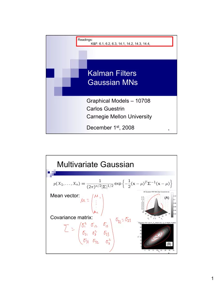

Readings: K&F: 6.1, 6.2, 6.3, 14.1, 14.2, 14.3, 14.4, Kalman Filters Gaussian MNs Graphical Models – 10708 Carlos Guestrin Carnegie Mellon University December 1 st , 2008 1 Multivariate Gaussian Mean vector: Covariance matrix: 2 1
Conditioning a Gaussian Joint Gaussian: p(X,Y) ~ N ( µ ; Σ ) Conditional linear Gaussian: p(Y|X) ~ N ( µ Y|X ; σ 2 Y|X ) 3 Gaussian is a “Linear Model” Conditional linear Gaussian: p(Y|X) ~ N ( β 0 + β X; σ 2 ) 4 2
Conditioning a Gaussian Joint Gaussian: p(X,Y) ~ N ( µ ; Σ ) Conditional linear Gaussian: p(Y|X) ~ N ( µ Y|X ; Σ YY|X ) 5 Conditional Linear Gaussian (CLG) – general case Conditional linear Gaussian: p(Y|X) ~ N ( β 0 + Β X; Σ YY|X ) 6 3
Understanding a linear Gaussian – the 2d case Variance increases over time (motion noise adds up) Object doesn’t necessarily move in a straight line 7 Tracking with a Gaussian 1 p(X 0 ) ~ N ( µ 0 , Σ 0 ) p(X i+1 |X i ) ~ N ( Β X i + β ; Σ Xi+1|Xi ) 8 4
Tracking with Gaussians 2 – Making observations We have p(X i ) Detector observes O i =o i Want to compute p(X i |O i =o i ) Use Bayes rule: Require a CLG observation model p(O i |X i ) ~ N (W X i + v; Σ Oi|Xi ) 9 Operations in Kalman filter X 1 X 2 X 3 X 4 X 5 O 1 = O 2 = O 3 = O 4 = O 5 = Compute Start with At each time step t : Condition on observation Prediction (Multiply transition model) Roll-up (marginalize previous time step) I’ll describe one implementation of KF, there are others Information filter 10 5
Exponential family representation of Gaussian: Canonical Form 11 Canonical form Standard form and canonical forms are related: Conditioning is easy in canonical form Marginalization easy in standard form 12 6
Conditioning in canonical form First multiply: Then, condition on value B = y 13 Operations in Kalman filter X 1 X 2 X 3 X 4 X 5 O 1 = O 2 = O 3 = O 4 = O 5 = Compute Start with At each time step t : Condition on observation Prediction (Multiply transition model) Roll-up (marginalize previous time step) 14 7
Prediction & roll-up in canonical form First multiply: Then, marginalize X t : 15 What if observations are not CLG? Often observations are not CLG CLG if O i = Β X i + β o + ε Consider a motion detector O i = 1 if person is likely to be in the region Posterior is not Gaussian 16 8
Linearization: incorporating non- linear evidence p(O i |X i ) not CLG, but… Find a Gaussian approximation of p(X i ,O i )= p(X i ) p(O i |X i ) Instantiate evidence O i =o i and obtain a Gaussian for p(X i |O i =o i ) Why do we hope this would be any good? Locally, Gaussian may be OK 17 Linearization as integration Gaussian approximation of p(X i ,O i )= p(X i ) p(O i |X i ) Need to compute moments E[O i ] E[O i 2 ] E[O i X i ] Note: Integral is product of a Gaussian with an arbitrary function 18 9
Linearization as numerical integration Product of a Gaussian with arbitrary function Effective numerical integration with Gaussian quadrature method Approximate integral as weighted sum over integration points Gaussian quadrature defines location of points and weights Exact if arbitrary function is polynomial of bounded degree Number of integration points exponential in number of dimensions d Exact monomials requires exponentially fewer points For 2 d +1 points , this method is equivalent to effective Unscented Kalman filter Generalizes to many more points 19 Operations in non-linear Kalman filter X 1 X 2 X 3 X 4 X 5 O 1 = O 2 = O 3 = O 4 = O 5 = Compute Start with At each time step t : Condition on observation (use numerical integration ) Prediction (Multiply transition model, use numerical integration ) Roll-up (marginalize previous time step) 20 10
Canonical form & Markov Nets 21 What you need to know about Gaussians, Kalman Filters, Gaussian MNs Kalman filter Probably most used BN Assumes Gaussian distributions Equivalent to linear system Simple matrix operations for computations Non-linear Kalman filter Usually, observation or motion model not CLG Use numerical integration to find Gaussian approximation Gaussian Markov Nets Sparsity in precision matrix equivalent to graph structure Continuous and discrete (hybrid) model Much harder, but doable and interesting (see book) 22 11
Recommend
More recommend