Active Appearance Models Edwards, Taylor, and Cootes Presented by - PowerPoint PPT Presentation
Active Appearance Models Edwards, Taylor, and Cootes Presented by Bryan Russell Overview Overview of Appearance Models Combined Appearance Models Active Appearance Model Search Results Constrained Active Appearance Models
Active Appearance Models Edwards, Taylor, and Cootes Presented by Bryan Russell
Overview Overview of Appearance Models Combined Appearance Models Active Appearance Model Search Results Constrained Active Appearance Models
What are we trying to do? Formulate model to “interpret” face images – Set of parameters to characterize identity, pose, expression, lighting, etc. – Want compact set of parameters – Want efficient and robust model
Appearance Models Eigenfaces (Turk and Pentland, 1991) – Not robust to shape changes – Not robust to changes in pose and expression Ezzat and Poggio approach (1996) – Synthesize new views of face from set of example views – Does not generalize to unseen faces
First approach: Active Shape Model (ASM) Point Distribution Model
First Approach: ASM (cont.) Training: Apply PCA to labeled images New image – Project mean shape – Iteratively modify model points to fit local neighborhood
Lessons learned ASM is relatively fast ASM too simplistic; not robust when new images are introduced May not converge to good solution Key insight: ASM does not incorporate all gray-level information in parameters
Combined Appearance Models Combine shape and gray-level variation in single statistical appearance model Goals: – Model has better representational power – Model inherits appearance models benefits – Model has comparable performance
How to generate a CAM Label training set with landmark points representing positions of key features Represent these landmarks as a vector x Perform PCA on these landmark vectors
How to generate a CAM (cont.) We get: Warp each image so that each control point matches mean shape Sample gray-level information g Apply PCA to gray-level data
How to generate a CAM (cont.) We get: Concatenate shape and gray-level parameters (from PCA) Apply a further PCA to the concatenated vectors
How to generate a CAM (cont.) We get:
CAM Properties Combines shape and gray-level variations in one model – No need for separate models Compared to separate models, in general, needs fewer parameters Uses all available information
CAM Properties (cont.) Inherits appearance model benefits – Able to represent any face within bounds of the training set – Robust interpretation Model parameters characterize facial features
CAM Properties (cont.) Obtain parameters for inter and intra class variation (identity and residual parameters) – “explains” face
CAM Properties (cont.) Useful for tracking and identification – Refer to: G.J.Edwards, C.J.Taylor, T.F.Cootes. "Learning to Identify and Track Faces in Image Sequences“. Int. Conf. on Face and Gesture Recognition, p. 260-265, 1998. Note: shape and gray-level variations are correlated
How to interpret unseen example Treat interpretation as an optimization problem – Minimize difference between the real face image and one synthesized by AAM
How to interpret unseen example (cont.) Appears to be difficult optimization problem (~80 parameters) Key insight: we solve a similar optimization problem for each new face image Incorporate a-priori knowledge for parameter adjustments into algorithm
AAM: Training Offline: learn relationship between error and parameter adjustments Result: simple linear model
AAM: Training (cont.) Use multiple multivariate linear regression – Generate training set by perturbing model parameters for training images – Include small displacements in position, scale, and orientation – Record perturbation and image difference
AAM: Training (cont.) Important to consider frame of reference when computing image difference – Use shape-normalized representation (warping) – Calculate image difference using gray level vectors:
AAM: Training (cont.) Updated linear relationship: Want a model that holds over large error range Experimentally, optimal perturbation around 0.5 standard deviations for each parameter
AAM: Search Begin with reasonable starting approximation for face Want approximation to be fast and simple Perhaps Viola’s method can be applied here
Starting approximation Subsample model and image Use simple eigenface metric:
Starting approximation (cont.) Typical starting approximations with this method
AAM: Search (cont.) Use trained parameter adjustment Parameter update equation:
Experimental results Training: – 400 images, 112 landmark points – 80 CAM parameters – Parameters explain 98% observed variation Testing: – 80 previously unseen faces
Experimental results (cont.) Search results after initial, 2, 5, and 12 iterations
Experimental results (cont.) Search convergence: – Gray-level sample error vs. number of iterations
Experimental results (cont.) More reconstructions:
Experimental results (cont.)
Experimental results (cont.) Knee images: – Training: 30 examples, 42 landmarks
Experimental results (cont.) Search results after initial, 2 iterations, and convergence:
Constrained AAMs Model results rely on starting approximation Want a method to improve influence from starting approximation Incorporate priors/user input on unseen image – MAP formulation
Constrained AAMs Assume: – Gray-scale errors are uniform gaussian with variance – Model parameters are gaussian with diagonal covariance – Prior estimates of some of the positions in the image along with covariances
Constrained AAMs (cont.) We get update equation: where:
Constrained AAMs Comparison of constrained and unconstrained AAM search
Conclusions Combined Appearance Models provide an effective means to separate identity and intra-class variation – Can be used for tracking and face classification Active Appearance Models enables us to effectively and efficiently update the model parameters
Conclusions (cont.) Approach dependent on starting approximation Cannot directly handle cases well outside of the training set (e.g. occlusions, extremely deformable objects)
Recommend
More recommend
Explore More Topics
Stay informed with curated content and fresh updates.
