A Unified Regularized Group PLS Algorithm Scalable to Big Data - PowerPoint PPT Presentation
A Unified Regularized Group PLS Algorithm Scalable to Big Data Pierre Lafaye de Micheaux 1 , Benoit Liquet 2 , Matthew Sutton 3 21 October, 2016 1 CREST, ENSAI. 2 Universit e de Pau et des Pays de lAdour, LMAP . 3 Queensland Uninversity of
A Unified Regularized Group PLS Algorithm Scalable to Big Data Pierre Lafaye de Micheaux 1 , Benoit Liquet 2 , Matthew Sutton 3 21 October, 2016 1 CREST, ENSAI. 2 Universit´ e de Pau et des Pays de l’Adour, LMAP . 3 Queensland Uninversity of Technology, Brisbane, Australia. Big Data PLS Methods JSTAR 2016, Rennes 1/54
Contents 1. Motivation: Integrative Analysis for group data 2. Application on a HIV vaccine study 3. PLS approaches: SVD, PLS-W2A, canonical, regression 4. Sparse Models ◮ Lasso penalty ◮ Group penalty ◮ Group and Sparse Group PLS 5. R package: sgPLS 6. Regularized PLS Scalable to BIG-DATA 7. Concluding remarks Big Data PLS Methods JSTAR 2016, Rennes 2/54
Integrative Analysis Wikipedia. Data integration “involves combining data residing in dif- ferent sources and providing users with a unified view of these data. This process becomes significant in a variety of situations, which in- clude both commercial and scientific domains”. System Biology. Integrative Analysis: Analysis of heterogeneous types of data from inter-platform technologies. Goal. Combine multiple types of data: ◮ Contribute to a better understanding of biological mechanisms. ◮ Have the potential to improve the diagnosis and treatments of complex diseases. Big Data PLS Methods JSTAR 2016, Rennes 3/54
Example: Data definition p q X Y n n - n observations - n observations - p variables - q variables Big Data PLS Methods JSTAR 2016, Rennes 4/54
Example: Data definition p q X Y n n - n observations - n observations - p variables - q variables ◮ “Omics.” Y matrix: gene expression, X matrix: SNP (single nu- cleotide polymorphism). Many others such as proteomic, metabolomic data. Big Data PLS Methods JSTAR 2016, Rennes 4/54
Example: Data definition p q X Y n n - n observations - n observations - p variables - q variables ◮ “Omics.” Y matrix: gene expression, X matrix: SNP (single nu- cleotide polymorphism). Many others such as proteomic, metabolomic data. ◮ “Neuroimaging”. Y matrix: behavioral variables, X matrix: brain activity (e.g., EEG, fMRI, NIRS) Big Data PLS Methods JSTAR 2016, Rennes 4/54
Example: Data definition p q X Y n n - n observations - n observations - p variables - q variables ◮ “Omics.” Y matrix: gene expression, X matrix: SNP (single nu- cleotide polymorphism). Many others such as proteomic, metabolomic data. ◮ “Neuroimaging”. Y matrix: behavioral variables, X matrix: brain activity (e.g., EEG, fMRI, NIRS) ◮ “Neuroimaging Genetics.” Y matrix: DTI (Diffusion Tensor Imag- ing), X matrix: SNP Big Data PLS Methods JSTAR 2016, Rennes 4/54
Data: Constraints and Aims ◮ Main constraint: colinearity among the variables, or situation with p > n or q > n . But p and q are supposed to be not too large. Big Data PLS Methods JSTAR 2016, Rennes 5/54
Data: Constraints and Aims ◮ Main constraint: colinearity among the variables, or situation with p > n or q > n . But p and q are supposed to be not too large. ◮ Two Aims: 1. Symmetric situation. Analyze the association between two blocks of information. Analysis focused on shared information. Big Data PLS Methods JSTAR 2016, Rennes 5/54
Data: Constraints and Aims ◮ Main constraint: colinearity among the variables, or situation with p > n or q > n . But p and q are supposed to be not too large. ◮ Two Aims: 1. Symmetric situation. Analyze the association between two blocks of information. Analysis focused on shared information. 2. Asymmetric situation. X matrix= predictors and Y matrix= response variables. Analysis focused on prediction. Big Data PLS Methods JSTAR 2016, Rennes 5/54
Data: Constraints and Aims ◮ Main constraint: colinearity among the variables, or situation with p > n or q > n . But p and q are supposed to be not too large. ◮ Two Aims: 1. Symmetric situation. Analyze the association between two blocks of information. Analysis focused on shared information. 2. Asymmetric situation. X matrix= predictors and Y matrix= response variables. Analysis focused on prediction. ◮ Partial Least Square Family: dimension reduction approaches Big Data PLS Methods JSTAR 2016, Rennes 5/54
Data: Constraints and Aims ◮ Main constraint: colinearity among the variables, or situation with p > n or q > n . But p and q are supposed to be not too large. ◮ Two Aims: 1. Symmetric situation. Analyze the association between two blocks of information. Analysis focused on shared information. 2. Asymmetric situation. X matrix= predictors and Y matrix= response variables. Analysis focused on prediction. ◮ Partial Least Square Family: dimension reduction approaches ◮ PLS finds pairs of latent vectors ξ = Xu , ω = Yv with maximal covariance. e . g ., ξ = u 1 × SNP 1 + u 2 × SNP 2 + · · · + u p × SNP p ◮ Symmetric situation and Asymmetric situation. ◮ Matrix decomposition of X and Y into successive latent variables. Latent variables: are not directly observed but are rather inferred (through a mathematical model) from other variables that are observed (directly measured). Capture an underlying phenomenon (e.g., health). Big Data PLS Methods JSTAR 2016, Rennes 5/54
PLS and sparse PLS Classical PLS ◮ Output of PLS: H pairs of latent variables ( ξ h , ω h ) , h = 1 , . . . , H . ◮ Reduction method ( H << min ( p , q ) ). But no variable selection for extracting the most relevant (original) variables from each latent variable. Big Data PLS Methods JSTAR 2016, Rennes 6/54
PLS and sparse PLS Classical PLS ◮ Output of PLS: H pairs of latent variables ( ξ h , ω h ) , h = 1 , . . . , H . ◮ Reduction method ( H << min ( p , q ) ). But no variable selection for extracting the most relevant (original) variables from each latent variable. sparse PLS ◮ sparse PLS selects the relevant SNPs ◮ Some coefficients u ℓ are equal to 0 ξ h = u 1 × SNP 1 + × SNP 2 + × SNP 3 + · · · + u p × SNP p u 2 u 3 ���� ���� = 0 = 0 ◮ The sPLS components are linear combinations of the selected variables Big Data PLS Methods JSTAR 2016, Rennes 6/54
Group structures within the data ◮ Natural example: Categorical variables form a group of dummy variables in a regression setting. Big Data PLS Methods JSTAR 2016, Rennes 7/54
Group structures within the data ◮ Natural example: Categorical variables form a group of dummy variables in a regression setting. ◮ Genomics: genes within the same pathway have similar functions and act together in regulating a biological system. ֒ → These genes can add up to have a larger effect ֒ → can be detected as a group (i.e., at a pathway or gene set/module level). Big Data PLS Methods JSTAR 2016, Rennes 7/54
Group structures within the data ◮ Natural example: Categorical variables form a group of dummy variables in a regression setting. ◮ Genomics: genes within the same pathway have similar functions and act together in regulating a biological system. ֒ → These genes can add up to have a larger effect ֒ → can be detected as a group (i.e., at a pathway or gene set/module level). We consider that variables are divided into groups: ◮ Example: p SNPs grouped into K genes ( X j = SNP j ) � � X = SNP 1 , . . . , SNP k | SNP k + 1 , SNP k + 2 , . . . , SNP h | . . . | SNP l + 1 , . . . , SNP p � ��������������� �� ��������������� � � �������������������������������� �� �������������������������������� � � ������������������ �� ������������������ � gene 1 gene 2 gene K ◮ Example: p genes grouped into K pathways/modules ( X j = gene j ) � � X = X 1 , X 2 , . . . , X k | X k + 1 , X k + 2 , . . . , X h | . . . | X l + 1 , X l + 2 , . . . , X p � ����������� �� ����������� � � ������������������ �� ������������������ � � ����������������� �� ����������������� � M 1 M 2 M K Big Data PLS Methods JSTAR 2016, Rennes 7/54
Group PLS Aim: select groups of variables taking into account the data structure Big Data PLS Methods JSTAR 2016, Rennes 8/54
Group PLS Aim: select groups of variables taking into account the data structure ◮ PLS components ξ h = u 1 × X 1 + u 2 × X 2 + u 3 × X 3 + · · · + u p × X p ◮ sparse PLS components (sPLS) ξ h = u 1 × X 1 + × X 2 + × X 3 + · · · + u p × X p u 2 u 3 ���� ���� = 0 = 0 Big Data PLS Methods JSTAR 2016, Rennes 8/54
Recommend
More recommend
Explore More Topics
Stay informed with curated content and fresh updates.
