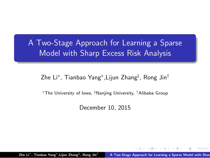
A Two-Stage Approach for Learning a Sparse Model with Sharp Excess - PowerPoint PPT Presentation

A Two-Stage Approach for Learning a Sparse Model with Sharp Excess Risk Analysis Zhe Li ∗ , Tianbao Yang ∗ ,Lijun Zhang ♮ , Rong Jin † ∗ The University of Iowa, ♮ Nanjing University, † Alibaba Group December 10, 2015 Zhe Li ∗ , Tianbao Yang ∗ ,Lijun Zhang ♮ , Rong Jin † A Two-Stage Approach for Learning a Sparse Model with Sharp

Problem Let x ∈ R d and y ∈ R denote an input and output pair Let w ∗ be an optimal model that minimizes the expected error 1 2 E P [( w T x − y ) 2 ] w ∗ = arg min || w || 1 ≤ B Key Problem : w ∗ is not necessarily sparse The goal : to learn a sparse model w to achieve small excess risk ER ( w , w ∗ ) = E P [( w T x − y ) 2 ] − E P [( w T ∗ x − y ) 2 ] ≤ ǫ Zhe Li ∗ , Tianbao Yang ∗ ,Lijun Zhang ♮ , Rong Jin † A Two-Stage Approach for Learning a Sparse Model with Sharp

The challenges L = E P [( w T x − y ) 2 ] is not necessarily strongly convex Stochastic optimization: O (1 /ǫ 2 ) sample complexity and no sparsity guarantee Empirical risk minimization + ℓ 1 penalty: O (1 /ǫ 2 ) sample complexity and no sparsity guarantee Challenges: Can we reduce sample complexity (e.g. O (1 /ǫ ))? Can we also have a guarantee on sparsity of model? Our solution: Zhe Li ∗ , Tianbao Yang ∗ ,Lijun Zhang ♮ , Rong Jin † A Two-Stage Approach for Learning a Sparse Model with Sharp

The first stage Our first stage algorithm is motivated by EPOCH-GD algorithm [Hazan, Kale 2011], which is on strongly convex setting. How to avoid strongly convex assumption? L ( w ) = E P [( w T x − y ) 2 ] = h ( Aw ) + b T w + c h ( · ): a strongly convex function The optimal solution set is a polyhedron By Hoffmans’ bound we have 2( L ( w ) − L ∗ ) ≥ 1 κ || w − w + || 2 2 where w + is the closest solution to w in the optimal solution set. [1] Elad Hazan, Satyen Kale, Beyond the regret minimization barrier: optimal algorithm for stochastic strongly-convex optimization Zhe Li ∗ , Tianbao Yang ∗ ,Lijun Zhang ♮ , Rong Jin † A Two-Stage Approach for Learning a Sparse Model with Sharp

The second stage Our second stage algorithm: Randomized Sparsification For k = 1 , . . . , K Sample i k ∈ [ d ] according to Pr( i k = j ) = p j w ik � Compute [ � w k ] i k = [ � w k − 1 ] i k + p ik End For � w 2 j E [ x 2 ˆ j ] | ˆ w j | p j = j ] instead of p j = w || 1 [Shalve-Shwartz et || ˆ � � d w 2 j E [ x 2 ˆ j =1 al., 2010] Reduced constant in O (1 /ǫ ) for sparsity [2] shalve-shwartz, Srebro, Zhang, Trading accuracy for sparsity in optimization problems with sparsity constraints Zhe Li ∗ , Tianbao Yang ∗ ,Lijun Zhang ♮ , Rong Jin † A Two-Stage Approach for Learning a Sparse Model with Sharp

Experimental Results E2006-tfidf E2006-tfidf E2006-tfidf 1.5 0.75 3 MG-Sparsification SpT: K = 500 Epoch-SGD 1.4 SGD DD-Sparsification SpS: B = 1 2.5 full model SpS: B = 2 1.3 SpS: B = 3 1.2 0.7 SpS: B = 4 2 RMSE RMSE RMSE SpS: B = 5 1.1 1.5 1 0.65 1 0.9 0.8 0.5 0.7 0.6 0 0.6 0 500 1000 1500 2000 2500 0 0.011 10.4 16.9 53.8 92.3 92.0 1 2 3 4 5 6 7 k K Sparsity(%) 1 st stage 2 nd stage RMSE vs Sparsity Zhe Li ∗ , Tianbao Yang ∗ ,Lijun Zhang ♮ , Rong Jin † A Two-Stage Approach for Learning a Sparse Model with Sharp