A Search and Jump Algorithm for Markov Chain Monte Carlo Sampling - PowerPoint PPT Presentation

A Search and Jump Algorithm for Markov Chain Monte Carlo Sampling Christopher Jennison Department of Mathematical Sciences, University of Bath, UK http://people.bath.ac.uk/mascj Adriana Ibrahim Institute of Mathematical Sciences, University of Malaya Seminar at University of Bath 22 November 2016 Chris Jennison and Adriana Ibrahim Search and Jump MCMC Sampling

Plan of talk 1. Basics of MCMC 2. The challenge: difficulties in getting a Markov chain to mix 3. Tjelmeland & Hegstad’s mode-jumping algorithm 4. A two-stage approach to mode-jumping 5. Example: Phosphate levels at an archaeological site 6. Example: Electron density in the ionosphere 7. Adapting the mode-jumping method to sample from distributions with “thin” support 8. Conclusions Chris Jennison and Adriana Ibrahim Search and Jump MCMC Sampling

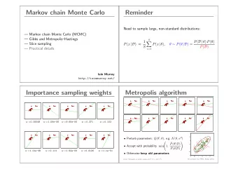
1. Markov chain Monte Carlo sampling (MCMC) Aim: To sample from a complex distribution π ( x ) on the state space Ω by running a Markov chain with limiting distribution π . Typically, X is high-dimensional and π not particularly tractable. The minimal requirement is that π ( x ) can be evaluated up to a multiplicative constant. Method: Create a Markov chain on Ω with transition matrix P satisfying π P = π. Let π n denote the distribution of the state X n after n transitions from an initial state x 0 . Then, if the Markov chain is irreducible and aperiodic, π n → π as n → ∞ . Chris Jennison and Adriana Ibrahim Search and Jump MCMC Sampling

A couple of comments (i) Notation: The distribution π ( x ) may be discrete or continuous. In the discrete case, the transition matrix P = ( P ij ) where P ij = P ( X n +1 = j | X n = i ) . In the continuous case, P ( x n , x n +1 ) specifies the conditional density of X n +1 given X n = x n . (ii) Generality: I shall describe methods and results for the continuous case. To obtain formulae for the discrete case, replace integrals by sums. Chris Jennison and Adriana Ibrahim Search and Jump MCMC Sampling

Detailed balance It is convenient to create a Markov chain with limiting distribution π by defining P to have detailed balance with respect to π , i.e., π ( x ) P ( x, y ) = π ( y ) P ( y, x ) for all x, y in Ω . The key property π P = π follows since � � π ( x ) P ( x, y ) dx = π ( y ) P ( y, x ) dx = π ( y ) . Ω Ω Examples of this construction are: Metropolis-Hastings samplers, based on the work of Metropolis et al. (1953) and Hastings (1970), The Gibbs sampler, introduced by Geman & Geman (1984). Chris Jennison and Adriana Ibrahim Search and Jump MCMC Sampling

The Metropolis-Hastings algorithm From X n = x , generate a proposal y from the kernel q ( x, y ) , Calculate the “acceptance probability” for this proposal α ( x, y ) = min { 1 , π ( y ) q ( y, x ) π ( x ) q ( x, y ) } , With probability α ( x, y ) , accept and move to X n +1 = y , With probability 1 − α ( x, y ) , reject and stay at X n +1 = x . Detailed balance: We need to show, for all x � = y , π ( x ) q ( x, y ) α ( x, y ) = π ( y ) q ( y, x ) α ( y, x ) . It is straightforward to check this holds for the two cases π ( x ) q ( x, y ) > π ( y ) q ( y, x ) and π ( x ) q ( x, y ) < π ( y ) q ( y, x ) . Chris Jennison and Adriana Ibrahim Search and Jump MCMC Sampling

The Gibbs sampler Suppose the sample space of the target distribution is Ω = R k . Let X ( − i ) denote the vector of elements of X excluding X ( i ) . Denote the conditional distribution of X ( i ) given X ( − i ) = x ( − i ) when X ∼ π by π X ( i ) | X ( − i ) ( x ( i ) | x ( − i )) . So π X ( i ) | X ( − i ) is a 1-dimensional PDF or discrete mass function. Denote by P i the transition matrix when X is modified by replacing X ( i ) with a new value sampled from π X ( i ) | X ( − i ) ( x ( i ) | x ( − i )) . In one cycle of the “Gibbs sampler”, X (1) , . . . , X ( k ) are updated in turn: the transition matrix for the full cycle is P = P 1 . . . P k . It is easy to show πP i = π for i = 1 , . . . , k and, hence, πP = π . Chris Jennison and Adriana Ibrahim Search and Jump MCMC Sampling

A variety of “move types” We may wish to use several “types” of move, indexed by a parameter φ ∈ Φ , with transition matrix P φ for move type φ . If each P φ satisfies detailed balance, we can deduce π P φ = π . Transitions can be made using a fixed sequence of move types φ . Alternatively, the move type for each transition may be selected at random (independently of the current state x ). In either case, the chain has limiting distribution π , as long as the chain is irreducible and aperiodic. We shall consider cases where one type of move produces small displacements in X , while other moves are designed to make larger jumps around the sample space Ω . Chris Jennison and Adriana Ibrahim Search and Jump MCMC Sampling

2. Mixing problems Efficient MCMC sampling needs π n to converge rapidly to π . Problem 1. Multiple modes 100 80 60 X(2) 40 20 0 0 20 40 60 80 100 X(1) To move between modes, updating one element of x at a time, requires a visit to a state with very low π ( x ) — and there is very little probability of accepting such a move. If updating several elements of x together, the proposal must land near the middle of the other mode in order to be accepted. Chris Jennison and Adriana Ibrahim Search and Jump MCMC Sampling

Mixing problems Problem 2. Very thin region of support for π 100 80 60 X(2) 40 20 0 0 20 40 60 80 100 X(1) Traversing the modal region of π with updates of X (1) and X (2) requires a great many small steps. Chris Jennison and Adriana Ibrahim Search and Jump MCMC Sampling

3. Mode jumping method of Tjelmeland & Hegstad (2001) Suppose the modes of π are small and in a high-dimensional space. We can create a proposal kernel q ( x, y ) that generates large jumps but the proposal y is unlikely to be at the centre of another mode. 100 80 60 X(2) y 40 x 20 0 0 20 40 60 80 100 X(1) The current state x will have fairly high π ( x ) but π ( y ) is small, so α ( x, y ) = min { 1 , π ( y ) q ( y, x ) π ( x ) q ( x, y ) } ≈ 0 . Chris Jennison and Adriana Ibrahim Search and Jump MCMC Sampling

The mode jumping method of Tjelmeland & Hegstad (2001) 100 y 80 x 2 60 X(2) x 1 +φ 40 x 20 0 0 20 40 60 80 100 X(1) T & H’s algorithm makes mode-jumping proposals by: 1. A large step from x to x 1 = x + φ , 2. Hill climbing from x 1 to x 2 , 3. Sample y from h ( x 2 , y ) , an approximation to π ( y ) at x 2 . Chris Jennison and Adriana Ibrahim Search and Jump MCMC Sampling

Achieving detailed balance in T & H’s algorithm 100 y 80 x 2 −φ y 1 60 X(2) x 1 +φ 40 y 2 x 20 0 0 20 40 60 80 100 X(1) 4. Construct a reverse step to y 1 = y − φ , 5. Hill climbing from y 1 to y 2 , 6. Fit a local approximation h ( y 2 , x ) to π ( x ) at y 2 , 7. Accept the move from x to y with probability α ( x, y ) = min { 1 , π ( y ) h ( y 2 , x ) π ( x ) h ( x 2 , y ) } . Chris Jennison and Adriana Ibrahim Search and Jump MCMC Sampling

T & H’s proof of detailed balance 100 y 80 x 2 −φ y 1 60 X(2) x 1 +φ 40 y 2 x 20 0 0 20 40 60 80 100 X(1) The “large step” move of type φ includes a random choice of + φ or − φ . In the proof of detailed balance, the forward move with + φ is paired with the reverse move with − φ and vice versa. Computationally, the return path has to be constructed in order to compute α ( x, y ) and accept or reject the proposal. The deterministic hill climbing step may be replaced by a stochastic optimisation step (Richard Sharp, University of Bath PhD Thesis). Chris Jennison and Adriana Ibrahim Search and Jump MCMC Sampling

T & H’s method: An example π ( x ) 1 / 5 In this 2-D distribution, both X (1) and X (2) range from 0 to 100 . Problems are likely to grow with X(2) X(1) dimensionality. The distribution to be sampled, π , has 7 highly compact modes, each bivariate normal or a transformed bivariate normal. Plotting π raised to the power 1 / 5 reduces the “spikiness” and makes a more meaningful plot. Chris Jennison and Adriana Ibrahim Search and Jump MCMC Sampling

T & H’s method: An example The support of each mode of π is very small — a standard MCMC sampler has very little chance of proposing a jump to a new mode. A specialised mode-jumping method is needed. We applied the T & H method with iterations comprising 20 local updates and 1 mode-jumping step. Local updates: Proposals have N (0 , 0 . 01 2 ) displacements in X (1) and X (2) . Mode jumping: Jumps have N (0 , 50 2 ) displacements in X (1) and X (2) , Quasi-Newton hill climbing using numerical second derivatives, Fitting a bivariate normal distribution at the top of the hill. Chris Jennison and Adriana Ibrahim Search and Jump MCMC Sampling

T & H’s method: An example 85.4 15.4 85.0 15.0 84.6 14.6 84.4 84.8 85.2 14.8 15.2 15.6 Mode 2 Mode 3 60.4 60.0 60.0 59.8 59.6 49.8 49.9 50.0 50.1 50.2 59.6 60.0 60.4 Mode 5 Mode 7 Details of the density of π (in colour) and the approximating bivariate normal density (in black) at four of the modes. Chris Jennison and Adriana Ibrahim Search and Jump MCMC Sampling