a) Rayleigh-Schrdinger perturbation theory b) choice of Hamiltonian - PowerPoint PPT Presentation

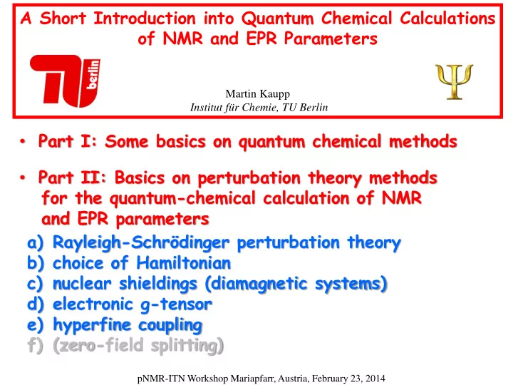
A Short Introduction into Quantum Chemical Calculations of NMR and EPR Parameters Martin Kaupp Institut für Chemie, TU Berlin • Part I: Some basics on quantum chemical methods • Part II: Basics on perturbation theory methods for the quantum-chemical calculation of NMR and EPR parameters a) Rayleigh-Schrödinger perturbation theory b) choice of Hamiltonian c) nuclear shieldings (diamagnetic systems) d) electronic g-tensor e) hyperfine coupling f) (zero-field splitting) pNMR-ITN Workshop Mariapfarr, Austria, February 23, 2014

A comprehensive treatment, Theory and Applications Wiley-VCH 2004. With 36 chapters on methodology and applications.

The effective spin Hamiltonian ˆ   H = E model structure   simulation properties spin Hamiltonian parameters Applications to: -spectra assignment -structure elucidation -interpretation comparison with model and/or -dynamics homologous systems ( e.g. from literature, database)

Introduction (1) effective spin Hamiltonian provides link between magnetic resonance experiment and quantum mechanical treatment:             H S g B S A I S D S I q I    N N   N ,         1        I B I D K I N N N NM NM M N N , M in most cases, property may be expressed as second derivative:   H ( , ) E a b     ( , ; , , ) X a S I b B S I     a b a b  appropriately treated by second-order perturbation theory:   0 V       ( , ) H H a b E

Introduction (2) -relation between effective-spin Hamiltonian and quantum-chemical treatment requires appropriate Hamiltonian that takes care of spins and magnetic fields  starting point relativistic quantum mechanics (e.g. Dirac equation) often transformation to quasi-nonrelativistic formalism (e.g. Breit-Pauli Hamiltonian) we will start by ignoring relativistic effects and magnetic interactions  initially nonrelativistic quantum mechanics for H 0 relativistic effects and magnetic interactions will be introduced later, mainly by perturbation theory

Part I: Some Basics on Quantum Chemical Methods

H 0 : Nonrelativistic Quantum Mechanics (1) The general (non-relativistic) Hamiltonian describing N electrons and M nuclei is given (in a.u.) by: 1 1 Z 1 Z Z                2 2 A A B H i A 2 2 M r r R         i 1 , N A 1 , M i 1 , N A 1 , M i 1 , N j i A 1 , M B A A iA ij AB

H 0 : Nonrelativistic Quantum Mechanics (2) after Born-Oppenheimer approximation (electronic Schrödinger equation):* electronic wave function ˆ    H E electron-electron electronic repulsion Hamiltonian 1 1   ˆ ˆ   H h ( i ) 2 r  i i j one-electron ij Hamiltonian 1 ˆ ˆ     2 h ( i ) ( i ) V ( i ) 2 operator of potential energy operator of kinetic energy (mainly el.-nuclear attraction) still missing: electronic spin (Pauli principle), *and time dependence removed

H 0 : Nonrelativistic Quantum Mechanics (3) energy expectation value:   H  E 0   variational principle: ~ ~   H ~   E E ~ ~ 0 0   exact ground-state solution provides lower bound to energies of approximate solutions!

H 0 : Nonrelativistic Quantum Mechanics (4) in the absence of electron-electron interactions:        ( 1 , 2 , 3 , 4 ,....... ) ( 1 ) ( 2 ) ( 3 ) ( 4 )..... ( ) n n 1 2 3 4 n Hartree product, independent-particle model, violates Pauli principle, no correlation.        ( 1 , 2 , 3 , 4 ,....... n ) ( 1 ) ( 2 ) ( 3 ) ( 4 )..... ( n ) 1 2 3 4 n Slater determinant (antisym. linear combination of product wavefunctions) -  i (i) : one-electron wave functions (molecular orbitals) -still no Coulomb correlation but Pauli exchange ~  insert as into variationa l principle !  Hartee-Fock method

H 0 : Nonrelativistic Quantum Mechanics (5) take trial wave function with free parameters q and minimize energy:* ~ ~   ~     H *Lagrange multipliers  a E     to account for constant 0 0 ~ ~ N(electrons), and for       q q orthogonality of MOs   for example: single Slater determinant  Hartree-Fock method       f ( 1 ) h ( 1 ) v ( 1 ) f ( 1 ) ( 1 ) ( 1 ) HF a a a 1 Z      2 A h ( 1 ) f depends on coordinates of 1 2 r A iA all electrons (via v HF )     ( 1 ) v J K iterative solution HF b b b     2 “self - consistent field” (SCF) method 1 J ( 1 ) dx ( 2 ) r b 2 b 12  i : molecular orbitals          * 1 K ( 1 ) ( 1 ) dx ( 2 ) r ( 2 ) ( 1 ) J i : Coulomb op., K i : exchange op. b a 2 b 12 a b

H 0 : Nonrelativistic Quantum Mechanics (6) algebraic expansion of  i into basis set: Roothan-Hall method  matrix operations, linear algebra     c ( A ) i ij j j optimizable parameters!!!  : atomic orbital basis function with center on atom A  MO expanded in linear combination of AOs  MO-LCAO method typical basis sets:           2   r r A f ( r , , ) e B g ( r , , ) e Gaussian-type orbitals (GTO) Slater-type orbitals (STO) integrals more convenient fullfil cusp condition others: plane waves, numerical AOs, muffin- tin orbitals, etc……* *also for DFT etc……..

H 0 : Nonrelativistic Quantum Mechanics (7) Hartree-Fock method accounts for Pauli exchange but not for Coulomb correlation  E HF  ~ E (even with infinite basis set!) 0 0 ~   HF E E E Löwdin definition of correlation energy corr 0 0  better methods (e.g. post-Hartree-Fock or DFT), to account for E corr post-HF methods: perturbation theory (MPn) size-consistent, not variational configuration interaction (CI) not size-consistent,* variational coupled-cluster theory (CC) size-consistent, not variational *in truncated form

A Hierarchy of post -Hartree-Fock Theories Semi-Empirical Density MO-Theory Functional Hartree-Fock (HF), SCF, MO-LCAO Theory ~        ( ) 1 ( )...... 2 ( n 1 ) ( ) n (n 3 -n 4 )  1 2 n 1 n n 4 Configuration Interaction (CI) Coupled Cluster Methods (CC) Perturbation Theory (MBPT)   ~ ~             ( C C r r C rs rs ......) e T (e.g. CCSD: n 6 , 0 0 a a ab ab 0 (e.g. MP2: n 5 , MP3: n 6 , MP4: n 7 )  r r s (       T T T CCSD(T): n 7 ) ........) (e.g. SDCI: n 6 ) 1 2 “Dressed CI Methods” CPF, ACPF, MCPF, CEPA typically n 6 Multiconfiguration SCF (MCSCF, CASSCF, GVB) Multireference Multireference Multireference Perturbation Theory Configuration Interaction Coupled Cluster Theory (CASPT2, MR-MP2, MR-MPn?) (e.g. MR-SDCI, MR-ACPF) n m : formal scaling factors relative to system size n. Note that linear pre-factors are also important

Density Functional Theory (1) basic idea: use r (r) instead of the more complicated y (r1,r2,….rn): Hohenberg-Kohn Theorem (1963): E = E [ r ] E [ r ] = T [ r ] + V ne [ r ] + V ee [ r ] =  r ( r )  ( r ) d r + F HK [ r ] Hohenberg-Kohn functional F HK [ r ] = T [ r ] + V ee [ r ] Kohn-Sham Method (1964): exchange-correlation F [ r ] = T s [ r ] + J [ r ] + E xc [ r ] functional of the KS method E xc [ r ] = T [ r ] - T s [ r ] + V ee [ r ] - J [ r ]

Density Functional Theory (2) Kohn-Sham equations:       f ( 1 ) ( 1 ) ( 1 ) f ( 1 ) h ( 1 ) v ( 1 ) a a a xc while formally similar to HF-SCF equations, KS method incorporates electron correlation via (unknown) v xc approximations to E xc and  xc : E xc r ]: local density approximation, LDA (e.g. SVWN, X  ) E xc r, r ]: gen. gradient approximation, GGA (e.g. BLYP, BP86, PW91, PBE,….) E xc r, r,  2 r, t ]: meta-GGA (e.g. PKZB, FT98,…..) hybrid functionals (with exact exchange) (e.g. B3LYP, BHPW91, mPW1,…) further: OEP, exact- exchange functionals….

Density Functional Theory (3) See also: https://sites.google.com/site/markcasida/dft Local Density Approximation (LDA) 1/3   3 3    r    r LDA LDA  4/3 r r r E ( ) d - d     (r) x x    4 E c for homogeneous electron gas not known analytically but from very accurate fits to Quantum Monte Carlo simulations Generalized Gradient Approximation (GGA)   r r  r GGA LDA   GGA    r r r r E ( ) F ( ), ( ) d     xc xc xc (different functionals have been constructed). Meta-Generalized Gradient Approximation (mGGA)     r  r  r t mGGA mGGA  2 r r r r E ( ), ( ), ( ), ( ) d r   xc xc 1 occ 2 t     r r ( ) ( ) i 2 i