A Monte-Carlo Option-Pricing Algorithm for Log-Uniform Jump-Diffusion - - PowerPoint PPT Presentation

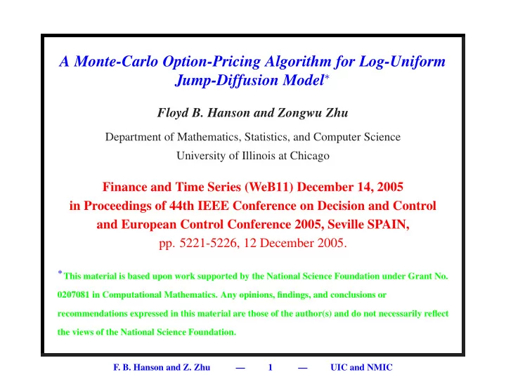
A Monte-Carlo Option-Pricing Algorithm for Log-Uniform Jump-Diffusion Model∗

Floyd B. Hanson and Zongwu Zhu

Department of Mathematics, Statistics, and Computer Science University of Illinois at Chicago

Finance and Time Series (WeB11) December 14, 2005 in Proceedings of 44th IEEE Conference on Decision and Control and European Control Conference 2005, Seville SPAIN,

• pp. 5221-5226, 12 December 2005.

∗This material is based upon work supported by the National Science Foundation under Grant No. 0207081 in Computational Mathematics. Any opinions, findings, and conclusions or recommendations expressed in this material are those of the author(s) and do not necessarily reflect the views of the National Science Foundation.

• F. B. Hanson and Z. Zhu

— 1 — UIC and NMIC

Overview

• 1. Introduction.
• 2. Risk-Neutral Constant-Coefficient Problems.
• 3. Risk-Neutral Option Price Solutions.
• Put-Call Parity.
• 4. Monte Carlo Algorithm.
• 5. Monte Carlo Simulation Results.
• 6. Conclusions.
• F. B. Hanson and Z. Zhu

— 2 — UIC and NMIC

• 1. Introduction

1.1 Background:

• Black-Scholes-Merton (2 seminal papers in Spring ’73 leading to ’97

Nobel Prize in Economics for Scholes and Merton, Black dying in ’95) option pricing formula is based upon a purely geometric (linear) diffusion process and its associated log-normal distribution.

• Statistical evidence that jumps are significant in financial markets:

– Stock and Option Prices in Ball and Torous (’85); – Capital Asset Pricing Model in Jarrow and Rosenfeld (’84); – Foreign Exchange and Stocks in Jorion (’89).

• F. B. Hanson and Z. Zhu

— 3 — UIC and NMIC

1.2 Market Jump Properties:

• Log-return market distributions usually skewed negative if data time

interval sufficiently long compared to the skew-less normal distribution.

• Log-return market distributions usually leptokurtic, i.e., more peaked

than the normal distribution.

• Log-return market distribution have fatter or heavier tails than the

normal distribution’s exponentially small tails.

• Stochastic dependence of volatility (standard deviation) is important.
• Time-dependence of rate coefficients is important, i.e., non-constant

coefficients are important.

• F. B. Hanson and Z. Zhu

— 4 — UIC and NMIC

1.3 Merton’s Jump-Diffusion Option Pricing Model:

• In Merton’s (’76) pioneering jump-diffusion option pricing model,

he used log-normally distributed jump-amplitudes in a compound Poisson process.

• Merton argued that the portfolio volatility could not be hedged as in

the Black-Scholes’ pure diffusion case, but that the risk-neutral property could preserve the no-arbitrage strategy by ensuring that the discounted, expected return would be at the market rate, all without relying on measure theory.

• Merton’s solution is the expected value of an infinite set of

Black-Scholes’ call option pricing formulas each one the initial stock price shifted by a jump factor depending on the number of jumps which have a Poisson distribution.

• F. B. Hanson and Z. Zhu

— 5 — UIC and NMIC

1.4 Risky Asset Stock Price, S(t), Dynamics at time t:

• Linear, Constant Rate Stochastic Differential Equation (SDE):

dS(t) = S(t)  µdt + σdW(t) +

dN(t)

• k=1

S(T −

k )J(Qk)

  , where S(0) = S0 > 0 and – µ = expected rate of return in absence of asset jumps, i.e., diffusive drift; – σ = diffusive volatility (standard deviation); – W (t) = Wiener (diffusion or Brownian motion) process, normally distributed such that E[W(t)] = 0 and Var[W(t)] = t; – J(Q) = Poisson jump-amplitude with underlying random mark variable Q, selected for log-return so that Q = ln(J(Q) + 1), such that J(Q) > −1; – N(t) = Poisson jump counting process, Poisson distributed such that E[N(t)] = λt = Var[N(t)];

• F. B. Hanson and Z. Zhu

— 6 — UIC and NMIC

1.4 Continued: Stock Price Dynamics: – T −

k is the pre-jump time and Qk is an independent and

identically distributed (IID) mark realization at the kth jump; – The processes W(t) and P(t) along with Qk are independent, except that Qk depends on a jump-event at Tk.

• Uniform Probability Jump-Amplitude Q Density:

φQ(q) = 1 b − a    1, a ≤ q ≤ b 0, else    , – Mark Mean µj ≡ EQ[Q] = 0.5(b + a); – Mark Variance σ2

j ≡ VarQ[Q] = (b − a)2/12;

– Jump-Amplitude Mean: ¯ J ≡E[J(Q)]≡E[exp(Q)−1]= (exp(b)−exp(a)) (b−a) −1.

• F. B. Hanson and Z. Zhu

— 7 — UIC and NMIC

1.5 Uniform Distribution Motivation:

• Extreme jumps in the market are relatively rare among the large

number of daily fluctuations and as statistical outliers they are very difficult, some say impossible, to include in statistical analysis of financial market data. With little information on the jump component, we focus here on the uniform jump-amplitude with the fattest of tails and finite range, that is consistent with the NYSE circuit breakers (since 1988) on extreme market changes.

• F. B. Hanson and Z. Zhu

— 8 — UIC and NMIC

1.6 Log-Return ln(S(t)) SDE and Solution:

• According to Itˆ
• ’s stochastic chain rule for jump-diffusions

d ln(S(t)) = (µ − σ2/2)dt + σdW(t) +

dN(t)

• k=1

Qk .

• Easily integrated in continuous and jump components:

S(t) = S0 exp  (µ − σ2/2)t + σW(t) +

N(t)

• k=1

Qk   . (1)

• F. B. Hanson and Z. Zhu

— 9 — UIC and NMIC

2. Risk-Neutral Constant-Coefficient Problems

First a critical theorem:

Theorem 2.1: Expected Jump-Diffusion Stock Price

E[S(t)] = S0 exp((µ + λ ¯ J)t), where S(t) is given in (1) and ¯ J. Proof: Using the mutual independence of the diffusion, Poisson counting and IID mark processes with separated and iterated expectations,

E[S(t)] = S0e(µ−σ2/2)tE » eσW (t)e

PN(t)

i=1 Qi

– = S0e(µ−σ2/2)tEW (t) h eσW (t)i EN(t) 2 4EQ|N 2 4

N(t)

Y

i=0

eQi ˛ ˛ ˛ ˛ ˛ ˛ N(t) 3 5 3 5 = S0e(µ−σ2/2)teσ2t/2

∞

X

k=0

pk(λt)

k

Y

i=0

EQ h eQii = S0e(µ+λ ¯

J)t,

where the Poisson distribution pk(λt) ≡ e−λt(λt)k/k! has been used.

• F. B. Hanson and Z. Zhu

— 10 — UIC and NMIC

2.2 Risk-Neutral Assumptions: After Merton’s discontinuous paper (1976),

• Jumps are due to Extreme Changes in Firm’s Specifics, i.e., Non-Systematic Risks,

e.g., bankruptcy, adverse legal rulings, unfavorable publicity, important discoveries, etc.

• Portfolio-Market Return Correlation beta (i.e., Cov[RS, RM]/Var[RM], where

return RX =∆X/X for X =S or M) is Zero and can be constructed by delta (i.e., ∂V/∂S) Hedging.

• Thus, Jump-Diffusion Model is Arbitrage-Free.
• ∴ Risk-Neutral World

= ⇒ E[S(t)] = S0 exp rt = ⇒ µ + λ ¯ J = r = ⇒ µ = µrn ≡ r − λ ¯ J. – Similarly, for time-dependent coefficients, µ(t) = µrn(t) ≡ r − λE[J(t, Q)].

• F. B. Hanson and Z. Zhu

— 11 — UIC and NMIC

2.3 Risk-Neutral Jump-Diffusion SDE:

Under Risk-Neutral Measure Mrn, in principle, dS(t)/S(t) =

• r−λ ¯

J

• dt+σdW(t)+

dN(t)

• k=1

J(Qk) = rdt+σdW(t) +

dN(t)

• k=1
• J(Qk)− ¯

J

• + ¯

J (dN(t)−λdt) , where jump terms are separated into the zero-mean forms of the compound Poisson process for convenience.

• F. B. Hanson and Z. Zhu

— 12 — UIC and NMIC

3. Risk-Neutral Option Price Solutions

3.1 Risk-Neutral European Call Option:

Under Risk-Neutral Valuation with Measure Mrn with drift µrn, the Payoff for European Call Option using Stock Price S(t) having exercise price K at exercise time T is C(S0, T) ≡ e−rT EM[max(S(T) − K, 0)] = e−rT √ 2π

∞

• k=0

pk(λT) kb

ka

∞

Z0(sk)

• S0eDJ(z,sk)−K
• ·e−z2/2φ e

Sk(sk)dzdsk

= 1 √ 2π

∞

• k=0

pk(λT)E e

Sk

∞

Z0( e Sk)

• S0eDJ(z, e

Sk))−rT − Ke−rT

·e−z2/2dz

• ,
• F. B. Hanson and Z. Zhu

— 13 — UIC and NMIC

3.1 Continued: Risk-Neutral Options: where the scaled jump-diffusion exponent is DJ(z, s)≡(r−λ ¯ J −σ2/2)T +σ √ Tz+s, the At-The-Money for standard normal integration variable is Z0(s)≡(ln(K/S0)−(r−λ ¯ J −σ2/2)T −s)/(σ √ T ) and the partial sum of k uniformly distributed IID marks is e Sk =

k

X

i=1

Qi

• n [a, b] and sk is the corresponding realized variable, such that e

S0 =P0

i=1Qi ≡ 0.

• F. B. Hanson and Z. Zhu

— 14 — UIC and NMIC

3.2 Black-Scholes Type Splitting of Integral: Let A(s) ≡ 1 √ 2π Z ∞

Z0(s)

S0e−(λ ¯

J+σ2/2)T +σ √ T z+se−z2/2dz

= S0es−λ ¯

JT Φ

“ d1 “ S0es−λ ¯

JT ””

, B(s) ≡ 1 √ 2π Z ∞

Z0(s)

Ke−rT e−z2/2dz =Ke−rT Φ “ d2 “ S0es−λ ¯

JT ””

, Φ(y)≡ 1 √ 2π Z y

−∞

e−z2/2dz is the standardized normal distribution and d1(x)≡(ln(x/K)+(r+σ2/2)T)/(σ √ T) & d2(x)≡d1(x) − σ √ T are the usual Black-Scholes normal distribution argument functions.

• F. B. Hanson and Z. Zhu

— 15 — UIC and NMIC

3.2 Continued: Splitting: ∴ C(S0, T) =

∞

X

k=0

pk(λT)E e

Sk

h A( e Sk)−B( e Sk) i =

∞

X

k=0

pk(λT)E e

Sk

» S0e

e Sk− λ ¯ JT Φ

“ d1 “ S0e

e Sk− λ ¯ JT ””

− Ke−rT Φ “ d2 “ S0e

e Sk− λ ¯ JT ””i

. =

∞

X

k=0

pk(λT)E e

Sk

h C(BS)“ S0e

e Sk−λ ¯ JT, T; K, σ2, r

”i , (2) where C(BS)(x, T; K, σ2, r)≡xΦ(d1(x))−Ke−rTΦ(d2(x)) is the Black-Scholes formula (1973), but with the stock price argument shifted by a jump factor exp( e Sk−λ ¯ JT).

• F. B. Hanson and Z. Zhu

— 16 — UIC and NMIC

3.3 Put-Call Parity Generally Valid:

Put-call parity is founded on basic maximum function properties (Merton (1973), Hull (2000) and Higham (2004)), so is independent of the particular process, C(S0, T) + Ke−rT = P(S0, T) + S0

• r solving for European put option price P(S0, T),

P(S0, T) = C(S0, T) + Ke−rT − S0, (3) assuming no dividends or transaction fees and that European call option price C(S0, T) is known.

• F. B. Hanson and Z. Zhu

— 17 — UIC and NMIC

4. Monte Carlo Simulations

For Monte Carlo simulations (e.g., see Glasserman (2004)), the European call option price formula (2) can be equivalently written compactly as C(S0, T) = E e

S(T )

• C(BS)

S0e

e S(T )−λ ¯ JT , T

• ,

(4) directly in terms of the compound Poisson process S(T)=N(T )

i=1 Qi with

uniformly distributed IID random variables Qi on [a, b]. Remark: If the zero mean process S(T)≡ S(T)−λ T ¯ J, where exp(λT ¯ J) = E[exp( S(T))], then exp( S(T)) is an exponential compound Poisson process with exponential martingale property on [0, T] that E[exp( S(T))]=exp( S(0))=1.

• F. B. Hanson and Z. Zhu

— 18 — UIC and NMIC

4.1 Compound Poisson Simulation Samples:

Let Ni be a IID Poisson variate sample point taken from the distribution

• f N(T) for i=1:n sample points. Given a jump in Ni, let Ui,j be IID

uniformly generated on [0, 1] sample points for j =1:Ni, then

• Si = Ni

j=1(a + (b − a)Ui,j) = aNi + (b − a) Ni j=1 Ui,j will be IID

compound Poisson random variables on [a, b] having the same distribution as S(T). An elementary Monte Carlo (EMC) estimate for C(S0, T) is

• Cn = 1

n

n

• i=1

C(BS) S0e

b Si−λ ¯ JT , T

• ≡ 1

n

n

• i=1
• C(BS)

i

, such that the C(BS)

i

are IID random variables based on Si.

• F. B. Hanson and Z. Zhu

— 19 — UIC and NMIC

4.2 Variance Reduction Techniques: Antithetic Variates:

Variance reduction techniques can reduce the size of σ b

Cn at reasonable

computational cost. If Ui,j is uniformly distributed on [0, 1], then the

• Qi,j =a+(b − a)Ui,j are uniformly distributed (thetic) random

variables on [a, b], so are the antithetic counterparts

• Q(a)

i,j =a+(b − a)(1−Ui,j) and

S(a)

i

≡ (b + a)Ni − Si are IID random variables for i = 1:n having the same compound Poisson distribution as S(T). Let the thetic-antithetic averaged, Black-Scholes risk-neutral, discounted payoff be

Xi =0.5 “ b C(BS)

i

+ b C(aBS)

i

” , (5)

where the antithetic b

C(aBS)

i

≡ C(BS)(S0e

b S(a)

i

−λ ¯ JT, T) , for i = 1:n, with

thetic-antithetic averaged jump factor

Yi = 0.5 “ exp “ b Si ” + exp “ b S(a)

i

”” , (6)

So the antithetic and thetic variates can be use together to double the sample size without significant computational cost (Boyle (1977)).

• F. B. Hanson and Z. Zhu

— 20 — UIC and NMIC

4.3 Variance Reduction Techniques: Control Variates:

Since E[exp( b

Si(T))] = exp(λT ¯ J) from Theorem 2.1 and exp( b Si(T)) has

positive correlation with C(BS)

i

, so the control variates technique can also be used to reduce the variance of Monte Carlo estimation, working faster the higher the correlation. The antithetic variate and control variate variance reduction techniques can be combined, the control adjusted payoff is

Zi(α) = Xi − α · (Yi − exp(λT ¯ J)) , (7)

where (Yi−exp(λT ¯ J)) is the control deviation and α is an adjustable control parameter. The sample mean of Zi(α) produces the Monte Carlo estimator for C(S0, T ), since

Zn(α)≡Pn

i=1Zi(α)/n =Xn−α(Y n−exp(λT ¯

J)), is an unbiased estimation

with E[Zn(α)]=C(S0, T) using IID mean properties E[Xn]=E[Xi]=C(S0, T) and E[Y n]=E[Yi]=exp(λT ¯

J) from the proof

• f Thm. 2.1.
• F. B. Hanson and Z. Zhu

— 21 — UIC and NMIC

4.3 Continued: Combined Antithetic and Control Variates: The variance of Zn(α) is σ2

Z n(α)≡Var

ˆ Zn(α) ˜ =Var[Zi(α)]/n ,

following from IID property of the Zi(α). However,

Var[Zi(α)]=Var[Xi]−2αCov[Xi, Yi]+α2Var[Yi].

So, the optimal parameter α∗ to minimize Var[Zi(α)] is α∗ =Cov[Xi, Yi]/Var[Yi]. (8) Using this optimal parameter α∗,

Var[Z∗

i ] ≡ Var[Zi(α∗)]=

` 1 − ρ2

Xi,Yi

´ Var[Xi],

where ρXi,Yi is the correlation coefficient between Xi and Yi. We also know that

Var[Xi] = 1 2 “ 1+ρ b

C(BS)

i

, b C(aBS)

i

” Var h b C(BS)

i

i

because Var

h b C(aBS)

i

i =Var h b C(BS)

i

i

.

• F. B. Hanson and Z. Zhu

— 22 — UIC and NMIC

4.4 Estimation of Optimal Parameter α∗: In general, the parameter α∗ is not known exactly, so estimation is needed along with the following results. Lemma 4.1: Var » e

b Si +e b S(a)

i

– =2 “ eλT ˆ

J −2e2λT ¯ J +eλT (ea+b−1)”

, where ˆ J = (exp(2b) − exp(2a))/(2(b − a))−1 and ¯ J = (exp(b) − exp(a))/(b − a)−1. Proof: Follows from properties of the antithetic pair `

b Si, b S(a)

i

´ . Lemma 4.2: An unbiased estimator for α∗ is b α = n n − 1 XY n −XnY n σ2

Y

, (9) where Xn = Pn

i=1 Xi/n is the sample mean, simlarly for XY n and Y n.

Proof: Basically, the condition for an unbiased estimate E[b α] = α∗ can be shown to be true.

• F. B. Hanson and Z. Zhu

— 23 — UIC and NMIC

4.4 Continued: Estimation of α∗: Since b α depends on Yi for i = 1:n, the estimate b α of α∗ introduces a bias into the estimate

• f control adjusted payoff

b Zn≡ 1 n

n

X

i=1

Xi − b α 1 n

n

X

i=1

Yi − eλT ¯

J

! . (10)

Theorem 4.3: The estimate b Zn of C(S0, T) has bias Bn ≡E[ b Zn]−C(S0, T)=Cov[X, (2µY −Y ])Y ]]/(nσ2

Y ) = O(1/n),

where µY = E[Yi] = exp(λT ¯ J), σ2

Y = Var[Yi], Y has same distribution as Yi, for

i = 1:n. Proof: This follows from the IID property of {XiYi}. Remark: The corrected unbiased estimate to b Zn is b Zn = b Zn − b Bn, where b Bn= 1 n − 1 XY

′

n − XnY

′

n

σ2

Y

, (11) while Y

′

i =Yi(2µY −Yi), XY

′

n, Xn and Y

′

n are sample means.

• F. B. Hanson and Z. Zhu

— 24 — UIC and NMIC

4.5 Monte Carlo Algorithm:

Finally, our Monte Carlo algorithm with antithetic and control variates (ACV Monte Carlo) variance reduction techniques :

for i = 1:n Randomly generate Ni by Inverse Transform Method; Randomly generate IID Ui,j, j = 1:Ni; Set b Si = aNi + (b − a) PNi

j=1 Ui,j;

Set b S(a)

i

= (a + b)Ni − b Si; Set C(BS)

i

= C(BS) “ S0 exp “ b Si − λT ¯ J ” , T ” ; Set C(aBS)

i

= C(BS) “ S0 exp “ b S(a)

i

− λT ¯ J ” , T ” ; Set Xi = 0.5 “ C(BS)

i

+ C(aBS)

i

” ; Set Yi = 0.5 “ exp( b Si) + exp “ b S(a)

i

”” ; end %for i Compute b α according to (9); Set b Zn = 1

n

Pn

i=1 Xi − b

α( 1

n

Pn

i=1 Yi − eλT ¯ J);

Estimate bias b Bn according to (11); Get European call b Zn = b Zn − b Bn; Get European put b P by (3).

• F. B. Hanson and Z. Zhu

— 25 — UIC and NMIC

5. Monte Carlo Simulation Results Table 1: Elementary (no ACV) Monte Carlo Results (see Discussion)

σ K/S0 C P ǫ t (sec.) ǫ √ t 0.9 13.76 0.67 0.055 2.640 0.090 0.2 1.0 5.26 3.28 0.035 2.578 0.056 1.1 1.38 8.49 0.014 2.562 0.022 0.9 15.99 2.90 0.048 2.562 0.077 0.4 1.0 8.45 6.47 0.033 2.578 0.053 1.1 4.07 11.18 0.020 2.531 0.032 0.9 19.15 6.03 0.044 2.454 0.069 0.6 1.0 11.79 9.81 0.033 2.500 0.052 1.1 7.09 14.21 0.023 2.500 0.036 Option parameters: K = 100, r = 0.1, T = 0.2, λ = 64, a = −0.028, b = 0.026. Simulation count n = 10, 000. Here, ǫ = σ b

Cn = σ(BS)/√n.

• F. B. Hanson and Z. Zhu

— 26 — UIC and NMIC

Table 2: Improved ACV Monte Carlo Results (see Discussion)

σ K/S0 C P ǫ t (sec.) ǫ √ t 0.9 13.73 0.64 0.004 6.875 0.011 0.2 1.0 5.23 3.25 0.008 6.828 0.021 1.1 1.38 8.49 0.006 6.781 0.016 0.9 16.03 2.94 0.004 7.031 0.011 0.4 1.0 8.42 6.44 0.004 6.922 0.011 1.1 4.06 11.17 0.004 7.218 0.011 0.9 19.11 6.02 0.003 6.797 0.008 0.6 1.0 11.81 9.83 0.003 6.859 0.008 1.1 7.12 14.23 0.003 6.812 0.008 Option parameters: K = 100, r = 0.1, T = 0.2, λ = 64, a = −0.028, b = 0.026. Simulation count n = 10, 000. Here, ǫ = σ b

Zn = σZ/√n.

• F. B. Hanson and Z. Zhu

— 27 — UIC and NMIC

5. Continued: Discussion of Table 1 and 2 Results:

• Table 1 and Table 2 show that the ACV Monte Carlo reduces the

standard error ǫ by a factor ranging from 2 to about 14, but increases the computing time by 2 to 3 times. However, a better benchmark trade-off is ǫ √ t, (Boyle, Broadie and Glasserman (1997)).

• Results show that the European call C option price is an increasing

function of initial stock price, S0 and the European put P is a decreasing function of S0.

• Both the call C and put P option prices increase with volatility σ.
• The estimated model parameters used for following Table 3 are

µ=0.1626, σ=0.1074, λ=64.16, a=−0.028, b=0.026 from our double-unform distribution paper (Zhu and Hanson (2005)) to compute the Standard & Poor 500 index option prices.

• F. B. Hanson and Z. Zhu

— 28 — UIC and NMIC

Table 3: Comparison of Option Prices by ACV Monte Carlo (see Discussion)

K S0

C P ǫ C(BS) P(BS) C∗ P∗ 0.8 269.81 0.01 2.e-3 269.80 2.e-6 269.82 0.02 0.9 132.36 1.45 0.03 130.98 0.07 132.39 1.47 1.0 40.07 20.27 0.11 30.49 10.69 40.05 20.25 1.1 5.49 76.60 0.06 1.13 72.24 5.50 76.61 1.2 0.31 147.17 0.01 4.e-3 146.87 0.32 147.19 Option parameters: K = 1000, r = 0.1, T = 0.2. S&P 500 estimated parameters: σ = 0.1074, λ = 64, a = −0.028, b = 0.026. Simulation count n = 10, 000. Here, ǫ = σ b

Zn = σZ/√n. The C∗ and P∗ values are obtained by more simulations, say

n = 400, 000 sample points, as a good approximation of the true values.

• F. B. Hanson and Z. Zhu

— 29 — UIC and NMIC

5. Continued2: Discussion of Table 3 Results:

• Computation of Black-Scholes call price C(BS)(S0, T; K, σ2, r) and

put price P(BS)(S0, T; K, σ2, r)=C(BS)(S0, T; K, σ2, r)+K exp(−rT)−S0

• nly gives a rough estimation of the true values.
• Table 3 shows that the estimated call C and put P values by ACV

Monte Carlo are within the 95% confidence interval of the approximate true call C∗ and put P∗ values, i.e., C ∈ [C∗ − 1.96ǫ, C∗ + 1.96ǫ] or P ∈ [P∗ − 1.96ǫ, P∗ + 1.96ǫ] by the central limit theorem.

• Theorem 5.1 Jump-Diffusion European option prices are bigger

than Black-Scholes option prices, independent of the Q-mark distribution, i.e., C(S0, T; K, σ2, r) ≥ C(BS)(S0, T; K, σ2, r), and P(S0, T; K, σ2, r) ≥ P(BS)(S0, T; K, σ2, r).

• F. B. Hanson and Z. Zhu

— 30 — UIC and NMIC

6. Conclusions

• Formulated a Risk-Neutral SDE appropriate for Compound

Jump-Diffusions, with emphasis on log-uniformly distributed jump-amplitudes.

• Antithetic and Control Variates (ACV) Monte Carlo is a

significant improvement of the elementary (no ACV) Monte Carlo lacking these variance reduction techniques.

• Jump-diffusion option prices are bigger than pure-diffusion

Black-Scholes option prices.

• Framework of ACV Monte Carlo option pricing algorithm is quite

general and can easily be applied to other jump-diffusion models.

• F. B. Hanson and Z. Zhu

— 31 — UIC and NMIC