A Framework for Adaptive Inflation and Covariance Localization for - PowerPoint PPT Presentation

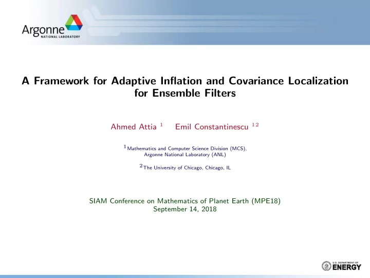
A Framework for Adaptive Inflation and Covariance Localization for Ensemble Filters Ahmed Attia 1 Emil Constantinescu 12 1 Mathematics and Computer Science Division (MCS), Argonne National Laboratory (ANL) 2 The University of Chicago, Chicago, IL SIAM Conference on Mathematics of Planet Earth (MPE18) September 14, 2018

Outline Ensemble Filtering Ensemble Kalman Filter (EnKF) Inflation & Localization Optimal Experimental Design OED and the alphabetical criteria OED Inflation & Localization A-OED inflation A-OED localization Numerical Experiments Experimental setup Numerical Results Adaptive Inflation and Localization [1/36] September 14, 2018: SIAM-MPE 18; Ahmed Attia.

Outline Ensemble Filtering Ensemble Kalman Filter (EnKF) Inflation & Localization Optimal Experimental Design OED and the alphabetical criteria OED Inflation & Localization A-OED inflation A-OED localization Numerical Experiments Experimental setup Numerical Results Adaptive Inflation and Localization Ensemble Filtering [2/36] September 14, 2018: SIAM-MPE 18; Ahmed Attia.

Ensemble Kalman Filter (EnKF) Assimilation cycle over [ t k − 1 , t k ] ; Forecast step ◮ Initialize: an analysis ensemble { x a k − 1 ( e ) } e =1 ,..., N ens at t k − 1 ◮ Forecast: use the discretized model M tk − 1 → tk to generate a forecast ensemble at t k : x b k ( e ) = M tk − 1 → tk ( x a k − 1 ( e )) + η k ( e ) , e = 1 , . . . , N ens ◮ Forecast/Prior statistics : � N ens 1 x b x b k = k ( e ) N ens e =1 � � T ; 1 N ens − 1 X b X b X b k = [ x b k (1) − x b k , . . . , x b k ( N ens ) − x b B k = k ] k k Forecast/Background Forecast/Background Ensemble ~ * + , # Ensemble ~ * + , # Initial/Analysis Ensemble ~ & ' ( "#$ Forward Forward Model Model Model Model Model ! " #$% ,→ " # ! " #$% ,→ " # State State State Time Time Time " #(% " #(% ! "#$ " # " # Adaptive Inflation and Localization Ensemble Filtering [3/36] September 14, 2018: SIAM-MPE 18; Ahmed Attia.

Ensemble Kalman Filter (EnKF) Assimilation cycle over [ t k − 1 , t k ] ; Analysis step ◮ Given an observation y k at time t k ◮ Analysis: sample the posterior (EnKF update) � � − 1 K k = B k H T H k B k H T k + R k k � k ( e )) � x a k ( e ) = x b [ y k + ζ k ( e )] − H k ( x b k ( e ) + K k ◮ The posterior (analysis) error covariance matrix : A k = ( I − K k H ) B k ≡ � � − 1 B − 1 + H T k R − 1 H k k Analysis Ensemble Analysis Ensemble Corrected Corrected ~ * + , # ~ * + , # Model State Model State (Analysis) (Analysis) Observation: ) # ; Likelihood: * ) # |, # Observation Observation Observation & & & Likelihood Likelihood Likelihood Forward Forward Forward Model Model Model Model Model Model ! " #$% ,→ " # ! " #$% ,→ " # ! " #$% ,→ " # State State State Time Time Time " #(% " #(% " #(% " # " # " # Adaptive Inflation and Localization Ensemble Filtering [4/36] September 14, 2018: SIAM-MPE 18; Ahmed Attia.

Ensemble Kalman Filter (EnKF) Sequential EnKF Issues ◮ Limited-size ensemble results in sampling errors, explained by: - variance underestimation - accumulation of long-range spurious correlations - filter divergence after a few assimilation cycles ◮ EnKF requires inflation & localization Sequentially Sequentially Repeat the Assimilation Cycle Repeat the Assimilation Cycle Assimilation Cycle Assimilation Cycle Analysis Ensemble Analysis Ensemble Corrected Corrected ~ , - . # ~ , - . # Model State Model State (Analysis) (Analysis) Forward Forward Observation Observation Model Model & & ! " # ,→ " #*% ! " # ,→ " #*% Likelihood Likelihood Forward Forward Model Model Model Model ! " #$% ,→ " # ! " #$% ,→ " # State State Time Time " #(% " #(% " # " # " #)% " #)% Adaptive Inflation and Localization Ensemble Filtering [5/36] September 14, 2018: SIAM-MPE 18; Ahmed Attia.

Ensemble Kalman Filter (EnKF) Inflation & Localization ◮ Covariance underestimation in EnKF is counteracted, by applying covariance inflation: → replace B , with an inflated version � B ◮ Long-range spurious correlations are reduced by covariance localization (e.g., Schur-product) → replace B , with a decorrelated version � B Adaptive Inflation and Localization Ensemble Filtering [6/36] September 14, 2018: SIAM-MPE 18; Ahmed Attia.

EnKF: Inflation ◮ Additive Inflation: s.t. D = diag ( λ ) , λ = � � T , 0 ≤ λ l � i ≤ λ i ≤ λ u B := D + B ; λ 1 , λ 2 , . . . , λ N state ◮ Multiplicative Inflation: 1. Space-independent inflation: X b = � √ λ � x b (1) − x b � λ � x b ( N ens ) − x b �� √ � ; 0 < λ l ≤ λ ≤ λ u , . . . , X b Ä � X b ä T 1 N ens − 1 � � B = = λ B 2. Space-dependent inflation: Let D := diag ( λ ) ≡ � N state λ i e i e T i , i =1 � 1 2 X b , X b = D X b Ä � X b ä T 1 1 1 N ens − 1 � � B = = D 2 BD 2 . ◮ The inflated Kalman gain � K , and analysis error covariance matrix � A BH T � BH T + R � − 1 ; A = � KH � � B ≡ �� B − 1 + H T R − 1 H � − 1 K = � � H � � I − � Adaptive Inflation and Localization Ensemble Filtering [7/36] September 14, 2018: SIAM-MPE 18; Ahmed Attia.

EnKF: Schur-Product Localization State-space formulation; B − Localization ◮ space-independent covariance localization: � B := C ⊙ B ; s.t. C = [ ρ i,j ] i,j =1 , 2 ,..., N state ◮ Entries of C are created using space-dependent localization functions † : � � → Gauss: − d ( i, j ) 2 ρ i,j ( L ) = exp ; i, j = 1 , 2 , . . . , N state , 2 L 2 → 5th-order Gaspari-Cohn:  � d ( i,j ) � 5 � d ( i,j ) � 4 � d ( i,j ) � 3 � d ( i,j ) � 2  − 1 + 1 + 5 − 5 + 1 , 0 ≤ d ( i, j ) ≤ L � d ( i,j ) � 5 � d ( i,j ) � 4 � d ( i,j ) � 3 � d ( i,j ) � 2 − 5 � d ( i,j ) � � � 4 L 2 L 8 L 3 L ρ i,j ( L ) = 1 − 1 + 5 + 5 + 4 − 2 L , L ≤ d ( i, j ) ≤ 2 L  12 L 2 L 8 L 3 L L 3 d ( i,j ) 0 . 2 L ≤ d ( i, j ) † - d ( i, j ) : distance between i th and j th grid points - L : radius of influence, i.e. localization radius Adaptive Inflation and Localization Ensemble Filtering [8/36] September 14, 2018: SIAM-MPE 18; Ahmed Attia.

EnKF: Schur-Product Localization Space-dependent formulation; B − Localization ◮ Space-dependent radii, i.e., L ≡ L ( i, j ) : we need to define localization kernel C → Examples include † :   C r = [ ρ i,j ( l i )] i,j =1 , 2 ,..., N state      C c = ( C r ) T = [ ρ i,j ( l j )] i,j =1 , 2 ,..., N state     2 ( C r + C c ) = � 2 ρ i,j ( l i ) + ρ i,j ( l j ) �    1 1   i,j =1 , 2 ,..., N state  C d = � ρ i,j ( l min ( i,j ) ) � C :=  i,j =1 , 2 ,..., N state  C u = � ρ i,j ( l max ( i,j ) ) �      i,j =1 , 2 ,..., N state   2 ( C d + C u ) = � 2 ρ i,j ( l min ( i,j ) ) + ρ i,j ( l max ( i,j ) ) �   1 1    i,j =1 , 2 ,..., N state  C G = � �� ��  ρ i,j l i l j i,j =1 , 2 ,..., N state ◮ We focus here on the symmetric kernel: C := 1 2 ( C r + C c ) = 1 2 [ ρ i,j ( l i ) + ρ i,j ( l j )] i,j =1 , 2 ,..., N state † Ahmed Attia, and Emil Constantinescu. ”An Optimal Experimental Design Framework for Adaptive Inflation and Covariance Localization for Ensemble Filters.” arXiv preprint arXiv:1806.10655 (2018). Adaptive Inflation and Localization Ensemble Filtering [9/36] September 14, 2018: SIAM-MPE 18; Ahmed Attia.

EnKF: Schur-Product Localization Space-dependent formulation; R − Localization ◮ Localization in observation space ( R − localization): ◮ HB is replaced with ” HB = C loc , 1 ⊙ HB , where C loc , 1 = � � ρ o | m ; i = 1 , 2 , . . . N obs ; j = 1 , 2 , . . . N state i,j � ◮ HBH T can be replaced with HBH T = C loc , 2 ⊙ HBH T , where C loc , 2 ≡ C o | o = � � ρ o | o ; i, j = 1 , 2 , . . . N obs i,j - ρ o | m is calculated between the i th observation grid point and the j th model grid point. i,j - ρ o | o i,j is calculated between the i th and j th observation grid points. ◮ Assign radii to state grid points vs. observation grid points: - Let L ∈ R N obs to model grid points, and project to observations for C loc , 2 [hard/unknown] - Let L ∈ R N obs to observation grid points; [efficient; followed here] Adaptive Inflation and Localization Ensemble Filtering [10/36] September 14, 2018: SIAM-MPE 18; Ahmed Attia.

Inflation & Localization Tuning the parameters ◮ Tuning the inflation parameter/factors λ - Bayesian approach for adaptive inflation exists, and still requires improvements - mostly for uncorrelated observation errors ◮ Tuning the localization radii of influence L - adaptive localization approaches are limited, especially in the vertical - mostly for uncorrelated observation errors - expert knowledge, especially with observation system, is required - theory is lacking The parameters λ , L are generally tuned empirically! Adaptive Inflation and Localization Ensemble Filtering [11/36] September 14, 2018: SIAM-MPE 18; Ahmed Attia.