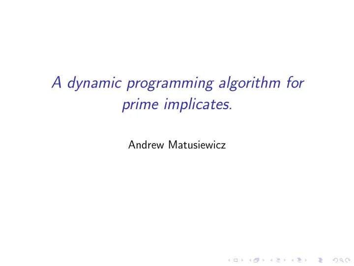
A dynamic programming algorithm for prime implicates. Andrew - PowerPoint PPT Presentation

A dynamic programming algorithm for prime implicates. Andrew Matusiewicz

What are prime implicates and why care? ◮ Smallest, simplest disjunctions implied by a statement

What are prime implicates and why care? ◮ Smallest, simplest disjunctions implied by a statement ◮ Knowing all prime implicates, clausal implication is easy

What are prime implicates and why care? ◮ Smallest, simplest disjunctions implied by a statement ◮ Knowing all prime implicates, clausal implication is easy ◮ Used in non-monotonic and abductive reasoning

What are prime implicates and why care? ◮ Smallest, simplest disjunctions implied by a statement ◮ Knowing all prime implicates, clausal implication is easy ◮ Used in non-monotonic and abductive reasoning ◮ Dual, prime implicants, used for circuit minimization

What are prime implicates and why care? ◮ Smallest, simplest disjunctions implied by a statement ◮ Knowing all prime implicates, clausal implication is easy ◮ Used in non-monotonic and abductive reasoning ◮ Dual, prime implicants, used for circuit minimization ◮ Research partner uses in code gen. for embedded systems (Sandeep Shukla, Virginia Tech.)

Propositional Clauses ◮ Propositional variables v 1 , v 2 , . . . are either true or false ◮ Connectives ∧ (and), ∨ (or), ¬ (not). ◮ A literal ℓ is a negated or non-negated variable: v i , ¬ v i ◮ A clause is an “or” of literals: ( v 1 ∨ ¬ v 3 ∨ v 2 ∨ v 9 ) = { v 1 , ¬ v 3 , v 2 , v 9 }

Prime Implicates A clause C is an “ implicate ” of a formula F iff the statement F ⇒ C is a tautology.

Prime Implicates A clause C is an “ implicate ” of a formula F iff the statement F ⇒ C is a tautology. C is a “ prime implicate ” of F , written C ∈ P ( F ) iff C is an implicate of minimal length.

Formulas as Graphs

Formulas as Graphs

Formulas as Graphs

“Tree-Like” formula ◮ Their graphs “resemble trees” at a macro level

“Tree-Like” formula ◮ Their graphs “resemble trees” at a macro level ◮ The common “closeness” measure to a tree is treewidth (Robertson and Seymour)

“Tree-Like” formula ◮ Their graphs “resemble trees” at a macro level ◮ The common “closeness” measure to a tree is treewidth (Robertson and Seymour) ◮ SAT instances F with fixed treewidth k may be solved in linear time.

Treewidth ◮ Synonyms for treewidth ◮ thin junction-tree or jointree (AI literature) ◮ k -tree embeddable (graph theory) ◮ triangularization, clique number k (Lauritzen and Spiegelhalter) ◮ channelwidth k (Hunt and Stearns) ◮ The channelwidth formalism is constructed for analysis of formulas ◮ Channelwidth uses objects called structure trees .

Structure Trees

Structure Trees

Structure Trees

Structure Trees

Structure Trees

Channel Variables ◮ Channel variables CV ( i ) of a node i are those that both

Channel Variables ◮ Channel variables CV ( i ) of a node i are those that both ◮ appear at or above that node

Channel Variables ◮ Channel variables CV ( i ) of a node i are those that both ◮ appear at or above that node ◮ appear in a clause at or below that node

Channel Variables ◮ Channel variables CV ( i ) of a node i are those that both ◮ appear at or above that node ◮ appear in a clause at or below that node ◮ The channelwidth of a formula is min S ∈ S max i ∈ I | CV ( i ) | where S is all valid structure trees for that formula

Channel Variables ◮ Channel variables CV ( i ) of a node i are those that both ◮ appear at or above that node ◮ appear in a clause at or below that node ◮ The channelwidth of a formula is min S ∈ S max i ∈ I | CV ( i ) | where S is all valid structure trees for that formula ◮ Channelwidth corresponds exactly to the graph theoretic notion of treewidth

Channel Variables

Properties of prime implicates ◮ With P 0 = P ( F [0 / v ]) and P 1 = P ( F [1 / v ]), we say S ( P 0 , P 1 , v ) = P ( F ) ( S runs in O ( n 4 ) time)

Properties of prime implicates ◮ With P 0 = P ( F [0 / v ]) and P 1 = P ( F [1 / v ]), we say S ( P 0 , P 1 , v ) = P ( F ) ( S runs in O ( n 4 ) time) ◮ If F and G share no variables and are satisfiable, P ( F ) ∪ P ( G ) = P ( F ∧ G )

Properties of prime implicates ◮ With P 0 = P ( F [0 / v ]) and P 1 = P ( F [1 / v ]), we say S ( P 0 , P 1 , v ) = P ( F ) ( S runs in O ( n 4 ) time) ◮ If F and G share no variables and are satisfiable, P ( F ) ∪ P ( G ) = P ( F ∧ G ) ◮ P (0) = { � } and P (1) = {}

Tables ◮ Let Γ( V ) be the set of interpretations of the variables V

Tables ◮ Let Γ( V ) be the set of interpretations of the variables V ◮ The table t for F with scope V is a mapping from Γ( V ) to clause sets such that t ( γ ) = P ( F [ γ ])

Tables ◮ Let Γ( V ) be the set of interpretations of the variables V ◮ The table t for F with scope V is a mapping from Γ( V ) to clause sets such that t ( γ ) = P ( F [ γ ]) ◮ Tables are determined exactly by their scope and formula

Tables ◮ Let Γ( V ) be the set of interpretations of the variables V ◮ The table t for F with scope V is a mapping from Γ( V ) to clause sets such that t ( γ ) = P ( F [ γ ]) ◮ Tables are determined exactly by their scope and formula ◮ Tables “split” the prime implicates of a formula along all interpretations of some of its variables

Obtaining tables ◮ For a structure tree S of F , let F i be the formula obtained by collecting all the clauses under node i .

Obtaining tables ◮ For a structure tree S of F , let F i be the formula obtained by collecting all the clauses under node i . ◮ Let T i be the table for F i with scope CV ( i )

Obtaining tables ◮ For a structure tree S of F , let F i be the formula obtained by collecting all the clauses under node i . ◮ Let T i be the table for F i with scope CV ( i ) ◮ We call T i “ i ’s table” or “the table of i ”

Obtaining tables ◮ If i is a leaf, T i can be obtained by the rules P (0) = { � } and P (1) = {}

Obtaining tables ◮ If i is a leaf, T i can be obtained by the rules P (0) = { � } and P (1) = {} ◮ If i is an internal node, T i can be obtained from the tables of i ’s children using the rules S ( P 0 , P 1 , v ) = P ( F ) and P ( F ) ∪ P ( G ) = P ( F ∧ G )

Obtaining tables ◮ If i is a leaf, T i can be obtained by the rules P (0) = { � } and P (1) = {} ◮ If i is an internal node, T i can be obtained from the tables of i ’s children using the rules S ( P 0 , P 1 , v ) = P ( F ) and P ( F ) ∪ P ( G ) = P ( F ∧ G ) ◮ Thus the table of any node may be obtained recursively.

Obtaining P ( F ) Let r be the root of S . Note that F r = F . ◮ Obtain T r recursively.

Obtaining P ( F ) Let r be the root of S . Note that F r = F . ◮ Obtain T r recursively. ◮ Narrow the scope of T r until it is empty, using S ( P 0 , P 1 , v ) = P ( F )

Obtaining P ( F ) ◮ A table r with scope ∅ results

Obtaining P ( F ) ◮ A table r with scope ∅ results ◮ The domain of this table is Γ( ∅ ), which contains only the empty assignment γ ∅

Obtaining P ( F ) ◮ A table r with scope ∅ results ◮ The domain of this table is Γ( ∅ ), which contains only the empty assignment γ ∅ ◮ r ( γ ∅ ) = P ( F r [ γ ∅ ])

Obtaining P ( F ) ◮ A table r with scope ∅ results ◮ The domain of this table is Γ( ∅ ), which contains only the empty assignment γ ∅ ◮ r ( γ ∅ ) = P ( F r [ γ ∅ ]) ◮ F r [ γ ∅ ] = F r = F

Obtaining P ( F ) ◮ A table r with scope ∅ results ◮ The domain of this table is Γ( ∅ ), which contains only the empty assignment γ ∅ ◮ r ( γ ∅ ) = P ( F r [ γ ∅ ]) ◮ F r [ γ ∅ ] = F r = F ◮ Thus r ( γ ∅ ) = P ( F )

Final words ◮ This is the first width-parameterized algorithm for prime implicate production

Final words ◮ This is the first width-parameterized algorithm for prime implicate production ◮ The task is still difficult with small treewidth, but this style of algorithm can prevent much repeated work.

Final words ◮ This is the first width-parameterized algorithm for prime implicate production ◮ The task is still difficult with small treewidth, but this style of algorithm can prevent much repeated work. ◮ Questions? Comments?