8 Neural MT 2: Attentional Neural MT In the past chapter, we - PDF document

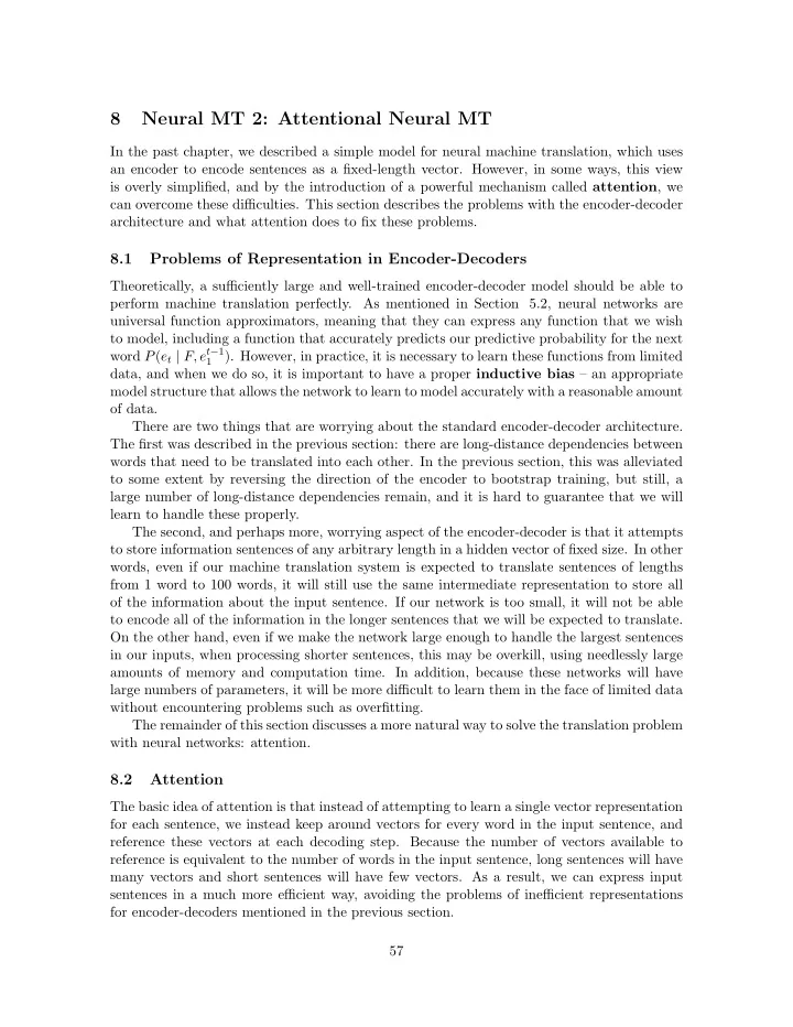
8 Neural MT 2: Attentional Neural MT In the past chapter, we described a simple model for neural machine translation, which uses an encoder to encode sentences as a fixed-length vector. However, in some ways, this view is overly simplified, and by the introduction of a powerful mechanism called attention , we can overcome these di ffi culties. This section describes the problems with the encoder-decoder architecture and what attention does to fix these problems. 8.1 Problems of Representation in Encoder-Decoders Theoretically, a su ffi ciently large and well-trained encoder-decoder model should be able to perform machine translation perfectly. As mentioned in Section 5.2, neural networks are universal function approximators, meaning that they can express any function that we wish to model, including a function that accurately predicts our predictive probability for the next word P ( e t | F, e t − 1 ). However, in practice, it is necessary to learn these functions from limited 1 data, and when we do so, it is important to have a proper inductive bias – an appropriate model structure that allows the network to learn to model accurately with a reasonable amount of data. There are two things that are worrying about the standard encoder-decoder architecture. The first was described in the previous section: there are long-distance dependencies between words that need to be translated into each other. In the previous section, this was alleviated to some extent by reversing the direction of the encoder to bootstrap training, but still, a large number of long-distance dependencies remain, and it is hard to guarantee that we will learn to handle these properly. The second, and perhaps more, worrying aspect of the encoder-decoder is that it attempts to store information sentences of any arbitrary length in a hidden vector of fixed size. In other words, even if our machine translation system is expected to translate sentences of lengths from 1 word to 100 words, it will still use the same intermediate representation to store all of the information about the input sentence. If our network is too small, it will not be able to encode all of the information in the longer sentences that we will be expected to translate. On the other hand, even if we make the network large enough to handle the largest sentences in our inputs, when processing shorter sentences, this may be overkill, using needlessly large amounts of memory and computation time. In addition, because these networks will have large numbers of parameters, it will be more di ffi cult to learn them in the face of limited data without encountering problems such as overfitting. The remainder of this section discusses a more natural way to solve the translation problem with neural networks: attention. 8.2 Attention The basic idea of attention is that instead of attempting to learn a single vector representation for each sentence, we instead keep around vectors for every word in the input sentence, and reference these vectors at each decoding step. Because the number of vectors available to reference is equivalent to the number of words in the input sentence, long sentences will have many vectors and short sentences will have few vectors. As a result, we can express input sentences in a much more e ffi cient way, avoiding the problems of ine ffi cient representations for encoder-decoders mentioned in the previous section. 57

Figure 25: An example of attention from [2]. English is the source, French is the target, and a higher attention weight when generating a particular target word is indicated by a lighter color in the matrix. First we create a set of vectors that we will be using as this variably-lengthed represen- tation. To do so, we calculate a vector for every word in the source sentence by running an RNN in both directions: � ! = RNN(embed( f j ) , � ! h ( f ) h ( f ) j − 1 ) j � = RNN(embed( f j ) , � h ( f ) h ( f ) j +1 ) . (68) j Then we concatenate the two vectors � ! and � h ( f ) h ( f ) into a bidirectional representation h ( f ) j j j = [ � j ; � ! h ( f ) h ( f ) h ( f ) j ] . (69) j We can further concatenate these vectors into a matrix: H ( f ) = concat col( h ( f ) 1 , . . . , h ( f ) | F | ) . (70) This will give us a matrix where every column corresponds to one word in the input sentence. We have a matrix H ( f ) with a variable However, we are now faced with a di ffi culty. number of columns depending on the length of the source sentence, but would like to use this to compute, for example, the probabilities over the output vocabulary, which we only know how to do (directly) for the case where we have a vector of input. The key insight of attention is that we calculate a vector α t that can be used to combine together the columns of H into a vector c t c t = H ( f ) α t . (71) 58

α t is called the attention vector , and is generally assumed to have elements that are between zero and one and add to one. The basic idea behind the attention vector is that it is telling us how much we are “fo- cusing” on a particular source word at a particular time step. The larger the value in α t , the more impact a word will have when predicting the next word in the output sentence. An ex- ample of how this attention plays out in an actual translation example is shown in Figure 25, and as we can see the values in the alignment vectors generally align with our intuition. 8.3 Calculating Attention Scores The next question then becomes, from where do we get this α t ? The answer to this lies in the decoder RNN, which we use to track our state while we are generating output. As before, the decoder’s hidden state h ( e ) is a fixed-length continuous vector representing the previous t , initialized as h ( e ) = h ( f ) target words e t − 1 | F | +1 . This is used to calculate a context vector c t 1 0 that is used to summarize the source attentional context used in choosing target word e t , and initialized as c 0 = 0 . First, we update the hidden state to h ( e ) based on the word representation and context t vectors from the previous target time step h ( e ) = dec([embed( e t − 1 ); c t − 1 ] , h ( e ) t − 1 ) . (72) t Based on this h ( e ) t , we calculate an attention score a t , with each element equal to a t,j = attn score( h ( f ) j , h ( e ) t ) . (73) attn score( · ) can be an arbitrary function that takes two vectors as input and outputs a score about how much we should focus on this particular input word encoding h ( f ) at the time step j h ( e ) t . We describe some examples at a later point in Section 8.4. We then normalize this into the actual attention vector itself by taking a softmax over the scores: α t = softmax( a t ) . (74) This attention vector is then used to weight the encoded representation H ( f ) to create a context vector c t for the current time step, as mentioned in Equation 71. We now have a context vector c t and hidden state h ( e ) for time step t , which we can pass t on down to downstream tasks. For example, we can concatenate both of these together when calculating the softmax distribution over the next words: p ( e ) = softmax( W hs [ h ( e ) t ; c t ] + b s ) . (75) t It is worth noting that this means that the encoding of each source word h ( f ) is considered j much more directly in the calculation of output probabilities. In contrast to the encoder- decoder, where the encoder-decoder will only be able to access information about the first encoded word in the source by passing it over | F | time steps, here the source encoding is accessed (in a weighted manner) through the context vector Equation 71. This whole, rather involved, process is shown in Figure 26. 59

this is a pen lookup lookup lookup lookup 0 RNN RNN RNN RNN RNN RNN RNN RNN 0 concat concat concat concat concat_col h t attn_score softmax x p t concat softmax(x+) Figure 26: A computation graph for attention. 8.4 Ways of Calculating Attention Scores As mentioned in Equation 73, the final missing piece to the puzzle is how to calculate the attention score a t,j . [8] test three di ff erent attention functions, all of which have their own merits: Dot product: This is the simplest of the functions, as it simply calculates the similarity between h ( e ) and h ( f ) as measured by the dot product: t j attn score( h ( f ) j , h ( e ) t ) := h ( f ) | h ( e ) (76) t . j This model has the advantage that it adds no additional parameters to the model. However, it also has the intuitive disadvantage that it forces the input and output encodings to be in the same space (because similar h ( e ) and h ( f ) must be close in space t j in order for their dot product to be high). It should also be noted that the dot product can be calculated e ffi ciently for every word in the source sentence by instead defining the attention score over the concatenated matrix H ( f ) as follows: attn score( H ( f ) , h ( e ) t ) := H ( f ) | h ( e ) (77) t . j Combining the many attention operations into one can be useful for e ffi cient impemen- tation, especially on GPUs. The following attention functions can also be calculated like this similarly. 29 Scaled dot product: One problem with the dot product is that it its value is highly de- pendent on the size of the hidden vector, with larger hidden vectors resulting in larger dot-product values (all else being equal). This can be problematic, because if the overall scale of the values going into the softmax function in Equation 74 are larger, then the 29 Question: What do the equations look like for the combined versions of the following functions? 60